
With COMSOL Multiphysics® version 6.1, we are happy to announce the release of a new interface that computes radiative loads on satellites in orbit. This Orbital Thermal Loads interface is part of the Heat Transfer Module and is used for defining satellite orbit and orientation, orbital maneuvers, and varying planetary properties. This interface is used to compute the solar, albedo, and Earth infrared thermal loads, which are then used to compute satellite temperature over time. Let’s learn more!
Background
Satellite thermal design is a challenging problem. A satellite is composed of many parts that can be sensitive to temperature: Sensors, cameras, radios, electronics, batteries, attitude control systems, and solar panels all need to be kept within certain temperature ranges, and even the satellite structure itself has to stay within certain temperature limits to prevent excessive thermal deformation. Heat dissipates from many of the components, and the satellite also experiences several different infrared (IR) thermal loads from the environment. Designing a satellite involves understanding how best to radiate all of this heat away and keep the satellite within desired operating conditions.
The heat generated by the various electronic components is usually quite simple to define, but the environmental loads can be surprisingly complex. First, there is the direct collimated solar flux incident on any surfaces facing the Sun. Next, for satellites in near-Earth orbits, the solar flux incident on the daylight side of the earth is diffusely reflected toward the earth-facing surfaces of the satellite. The magnitude of these reflections depends upon both the local surface properties of the earth as well as the changing atmospheric conditions. In total, the diffusely reflected solar flux is about one-third of the direct solar flux and is referred to as the albedo flux. When the satellite goes into eclipse, these direct solar and albedo loads drop to zero, but there is a third source of environmental heating that is always present: The earth is warm and acts as a diffuse radiator, with the magnitude of this planet IR radiation being a function of latitude as well as longitude.
Knowing these time-varying environmental fluxes, as well as their distribution over the satellite surfaces, is a needed input for computing the satellite temperature, which involves solving for the thermal conduction within the solid parts and the radiation from all exposed surfaces. It is common to divide these environmental fluxes into two bands: the solar band and the ambient band. The reason for this is that the Sun, at about 5780 K, emits predominantly short-wavelength radiation, while the satellite and the earth are both at about 300 K and emit predominantly longer wavelengths IR radiation. This division is important since the surface absorptive properties of the exterior coatings on the satellite are often specifically tailored to be a function of wavelength for the purposes of thermal management. For example, to keep the satellite’s operating temperature as low as possible, one approach is to use surface coatings with low absorptivity (emissivity) in the solar band but high emissivity in the ambient band.
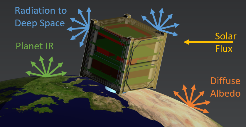
The radiative heat transfer experienced by a satellite in orbit depends upon its position and orientation relative to the earth and Sun. Earth image credit: Visible Earth and NASA.
A satellite of constant mass orbiting about a much more massive spherical planet follows an elliptical path, and this path can be described by the Keplerian orbital elements, which describe a periodic orbit. The orbital elements are used to compute (via the equation of the center) the coordinates of the satellite in the equatorial coordinate system (ECS).
Along with knowing the position of the satellite over time, it is also necessary to know how it is oriented. This begins by defining the satellite coordinate system via a set of satellite axes. Depending upon the mission parameters, these satellite axes are oriented toward particular directions, such as toward the earth, the Sun, the direction of travel, or a fixed point in the celestial sphere. It may also be desirable to change these axes’ definitions and their orientations, such as for the purpose of facing an instrument toward a geographic location. The satellite may also be rotating slowly about one or more axes or tumbling relatively rapidly. Changes in orientation affect the loads as well as the shadowing of the satellite. For example, a protrusion from the satellite, such as a solar panel or instrument, will shade the surfaces behind it. If there are rotating solar panels or other articulating elements, this will also alter the shading and loads. If the satellite is tumbling rapidly, on the other hand, this implies an averaging of the environmental loads.
Once all mission parameters are known, it is possible to compute all of the environmental loads, and it then becomes quite straightforward to compute the temperature profile of the satellite over time. Now, let us take a look through the Orbital Thermal Loads user interface and explore how it can help with all of these inputs when setting up a satellite thermal analysis.
Overview of the Orbital Thermal Loads User Interface
The Orbital Thermal Loads interface works similarly to any other interface within the COMSOL Multiphysics product suite and takes advantage of the uniform workflow. You start by either:
- Creating your own CAD description of the structure within the software using the core CAD modeling capabilities or the Design Module
- Importing from a CAD file, such as a Parasolid®, ACIS®, or STEP file
- Using one of the LiveLink™ for CAD products to bidirectionally link COMSOL® to your CAD platform
From here, you will use CAD simplification and cleanup and meshing, solving, and results evaluation functionality similar to any other workflow, so if you’re already a COMSOL user, you will get up to speed with this new interface very quickly.
As part of a typical workflow, the Orbital Thermal Loads interface is used in three steps, corresponding to three different study types. First, the orbital elements and the satellite axes and orientation are defined, and either one or several orbital periods are solved for using an Orbit Calculation study step. This lets us quickly verify the mission parameters before computing the irradiance from all environmental sources via the Orbit Thermal Loads study step. Once these irradiances are solved for and stored, they are used to compute the temperature of the structure and the surface-to-surface radiation between all exposed surfaces over time using the Orbital Temperature study step. For cases where the environmental loads are the same for each orbit, the loads can be computed for just one orbit and repeated in time for the thermal analysis.
The Orbital Thermal Loads interface can be used on its own to compute the environmental heat loads, but more typically it is used in conjunction with the Heat Transfer in Solids and Events interfaces. The Heat Transfer in Solids interface computes the temperature distribution within the solid structure of the satellite, and the Events interface keeps track of eclipses and reorientations, as well as any other instantaneous changes in the state, such as instruments turning on and off.
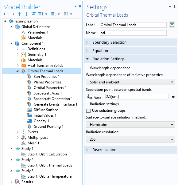
Screenshot showing the Orbital Thermal Loads interface, along with the three associated study types.
The settings for the interface are shown in the screenshot above and are similar to the settings for the Surface-to-Surface Radiation interface but instead use the Solar and ambient two-band model by default. Radiation is always present between all exposed surfaces, both exterior and interior to the satellite.
Now, let us look through the default features within the interface.
First the Sun Properties feature defines the direction of the incident sunlight in the ECS as well as the solar flux. Four predefined options are available for the Sun direction. The options are defined in terms of the equinoxes and solstices of the earth, which will control the Sun vector and solar flux. You can also enter your own Sun vector and make this a time-varying expression. If using a multiband spectral model, the Sun can be treated either as a blackbody emitter, as having a defined flux within each band, or via a distribution of flux as a function of wavelength. It is usually sufficient to treat the Sun as a blackbody emitter, which is the default behavior.
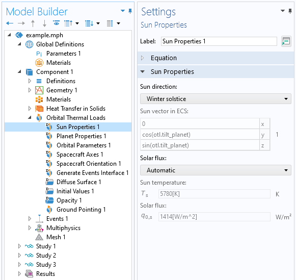
The Sun Properties feature specifies the orientation of the Sun vector and the solar flux.
Next, the Planet Properties feature specifies several parameters that are needed to compute the orbit and eclipses. The Planet longitude at start time orients the planet under the satellite and is important when orbital maneuvers are specified in terms of a location on the ground or when the planet properties are a function of latitude and longitude. The Radiative Properties section can be used to enable albedo and planet IR loads, and both the Albedo and Planet infrared flux can be made functions of latitude and longitude. These data can be read in from a spreadsheet or from image data. The planet is treated via a discretization whereby the visible part of the planet is subdivided into a set of patches with equal view factors. When the albedo or planet IR properties vary significantly, and for low-altitude orbits, a finer discretization may be needed.
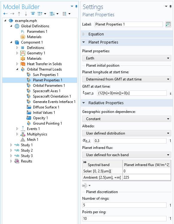
The Planet Properties feature orients the planet underneath the satellite at start time and describes the radiative properties of the planet.
The next default feature, Orbital Parameters, presents the settings to define the orbit in terms of the six Keplerian orbital elements of an elliptical orbit: semimajor axis, eccentricity, inclination, longitude of ascending node, argument of periapsis, and the true anomaly at start time. Circular, Elliptical Equatorial, and Circular Equatorial orbits can also be defined, in terms of a reduced set of parameters.
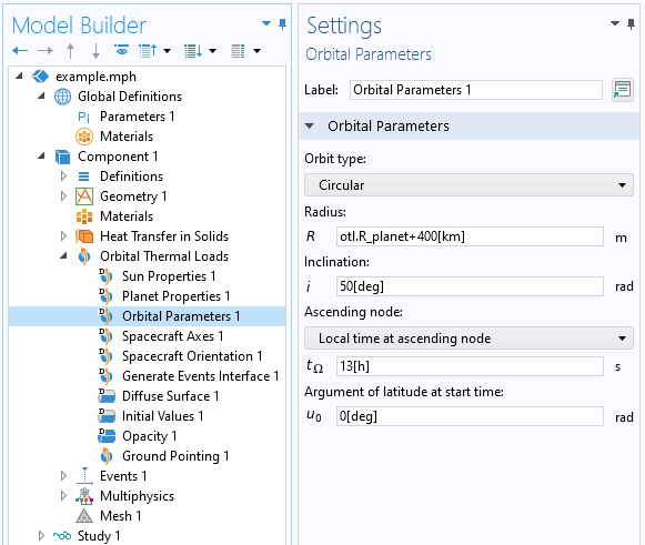
The Orbital Parameters feature is used to enter the orbital elements.
The Spacecraft Axes feature defines the axis directions of the satellite coordinate system. These axes can be specified in the CAD coordinates or by selecting a face of the satellite, in which case the face-normal direction is used. This is useful when pointing an instrument in a specific direction. The selected secondary pointing direction need not be perpendicular to the primary; the projection of the secondary vector onto the plane normal to the primary is taken. The third axis completes a right-handed coordinate system. It is possible to define different coordinate systems, which are used in conjunction with the Spacecraft Orientation feature.
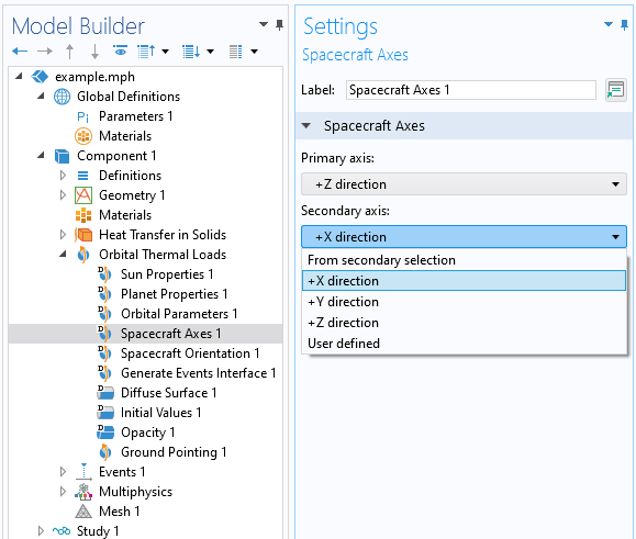
The Spacecraft Axes feature defines the primary and secondary pointing directions.
The Spacecraft Orientation feature defines the directions toward which the spacecraft’s primary and secondary axes are oriented, as well as the rotations, if any, about the primary, secondary, and third directions. The orientation directions can be any one of Zenith/Nadir, Sun/AntiSun, Velocity/Antivelocity, Orbit Normal/Antinormal, Celestial Point, or Ground Station. The satellite will exactly face the primary pointing direction and be rotated such that the secondary spacecraft pointing direction points toward the second orientation direction.
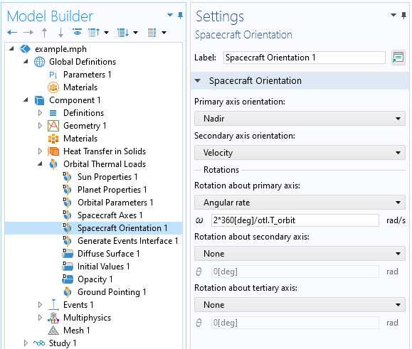
The Spacecraft Orientation feature, in conjunction with the Spacecraft Axes feature, defines how the satellite is positioned over time.
If there is only one each of the Spacecraft Axes and the Spacecraft Orientation features, then these are used throughout the analysis. It is possible to have multiple instances of these features — and to switch between them — to introduce a variety of orbital maneuvers. To switch between combinations of definitions, the Generate Events Interface feature is used, which allows for sequences of orbital maneuvers, such as pointing at a specific geographic location while the satellite is in range.
There is another purpose of the Events interface that is persistent across all use cases: The tracking of eclipses. The times when the satellite enters and leaves eclipse (if they occur) are used to indicate to the solver that a change in the thermal load is occurring.
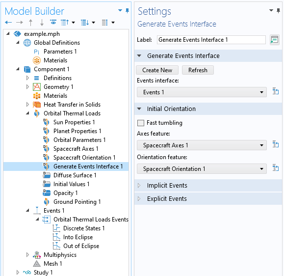
The Generate Events Interface feature will populate the Orbital Thermal Loads Events node within the Events interface. Eclipses are always considered.
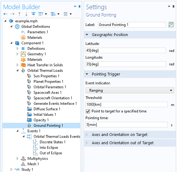
The Ground Pointing feature can be used to set up additional events that point the satellite toward a geographic location based upon different conditions.
The remaining features in the interface, the Diffuse Surface, Initial Values, and Opacity features, all relate to the modeling of the emission and reflection of the various modeled surfaces.
For a thermal modeling point of view, once the environmental loads are computed, the workflow is identical to any other model involving thermal conduction and radiation. The Orbital Thermal Loads interface solves for radiative heat transfer and is coupled to the Heat Transfer in Solids interface, which accounts for the thermal conduction within the solid structure of the satellite and also allows you to define thermal loads within volumes or surfaces that can either be constant or time-varying. Beyond this, you also have the complete feature set of the Heat Transfer Module, including:
- Conductive heat transfer in thin-walled parts
- Thermal contact resistance across interfaces
- Phase change materials
- Convective heat transfer in fluids
- Lumped thermal connections and components
Once you’ve fully defined the problem and have solved for the orbital thermal loads as well as the temperature, you’ll get a set of default plots, and you can also create any number of other visualizations of the data. Let’s look at some of these…
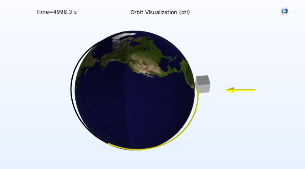
Plot showing the orbit around the earth, the Sun vector, and the orientation of the satellite. Earth image credit: Visible Earth and NASA.
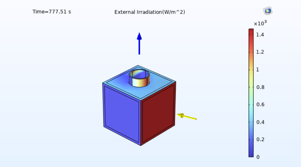
Plot of the total irradiation from all environmental sources, as well as the Sun vector over time and the Nadir direction.
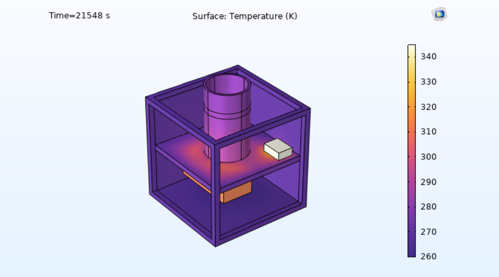
Plot showing the temperature of several components within a small satellite. Some external surfaces are hidden.
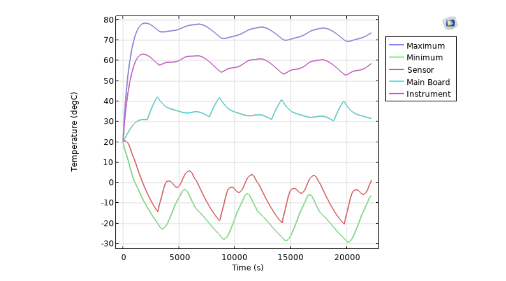
Plot of the temperature of a few components converging to a cycle-periodic state over several orbits.
Closing Remarks
With the new Orbital Thermal Loads interface, it is now possible to quickly set up a thermal model of a satellite in orbit to predict operational performance. The interface is a great tool for engineers working on the planning and design of a satellite. For those users of the Heat Transfer Module who would like to get started right away, see the following examples:
Editor’s note: You can learn more about the thermal modeling of small satellites in this Tech Briefs article by Walter Frei, published on January 1, 2023.
LiveLink is a trademark of COMSOL AB. Parasolid is a trademark or registered trademark of Siemens Product Lifecycle Management Software Inc. or its subsidiaries in the United States and in other countries. ACIS is a registered trademark of Spatial Corporation.


Comments (18)
Robert Luppold
December 9, 2022Excellent presentation of the physical phenomena and the modeling capabilities of the new COMSOL toolbox. Thank you for a job well done.
Salih KAYA
December 30, 2022hello, how can we define start time for satellite analysis? like December 21st
Walter Frei
December 30, 2022 COMSOL EmployeeHello Salih,
The Sun Properties allows you to define the sun vector (which is already set up for Winter Solstice) and within the Planet Properties, you can define the start time of day.
Salih KAYA
January 4, 2023thank you, in COMSOL, How to calculate the absorbed heat from solar loads inside the aircraft? absorption coefficient not entered in the video
Walter Frei
January 4, 2023 COMSOL EmployeeHello Salih,
Yes, it’s important to understand the concepts here:
https://www.comsol.com/blogs/modeling-emissivity-in-radiative-heat-transfer/
https://www.comsol.com/blogs/modeling-incident-radiation-in-radiative-heat-transfer/
https://www.comsol.com/blogs/introduction-to-computing-radiative-heat-exchange/
In short, though, emissivity equals absorptivity.
Salih KAYA
January 4, 2023thank you so much,
Best Regards
Wai Kwuen Choong
May 21, 2023Hi, Is that possible to neglect the internal radiative heat exchange when we are using orbital thermal load interface? It could really help in modeling a heavy satellite system in a preliminary design phase.
Walter Frei
May 22, 2023 COMSOL EmployeeHello Wai,
Yes, you can do this. The approach is to include only those faces that can see space, in the Orbital Thermal Loads interface. That way, radiation from all internal faces is neglected.
Best,
Walter
Wai Kwuen Choong
May 23, 2023Hi Walter, thank you.
I’m wondering how to simulate MLI (multi-layer insulation) in COMSOL, instead of set up ideally diffuse mirror, can we set up a diffuse surface with up (space-facing) and down (solid domain facing, setting effective emittance of MLI) optical properties on a boundary of a solid domain? When we are using up-and-down radiative properties in the boundary, how does the heat exchange in the boundary (boundary without assign material heat capacity)?
Best,
Ken
Walter Frei
May 24, 2023 COMSOL EmployeeHello Ken,
MLI can be a complicated topic, likely to vast to cover here at the level it deserves. If we think abut MLI in the context of the James Webb heat shield, then one should model each layer explicitly. On the other hand, for an MLI blanket that is extensively taped down, and in many places having contact between layers, where there can be thermal contact and conduction between layers, it’s more motivated to go with an experimental correlation for the equivalent (temperature dependent) conductivity of a thin layer on the solid model. More specific situations and guidance are better to discuss within the context of COMSOL Support.
Best,
Walter
Wai Kwuen Choong
May 25, 2023Hi Walter,
Great, I think we will go through an experimental correlation to get those properties,
and will soon discuss with COMSOL Support, thank you.
Best,
Ken
Salih Kaya
June 23, 2023Considering a satellite operating at 560 km altitude at SSO, I want to calculate the worst-cold case for thermal analysis. The assumptions for this case follows as: For the Sun Properties, Sun direction at winter solstice; Planet Properties for Earth as longitud facing the vernal point is 270 degrees to catch the winter solstice accordingly. I have a problem with determining the local time of the ascending node according to default GMT value of COMSOL (which I do not know), true solar time and mean solar time. Can you please elaborate on their relationship for the worst-cold case?
鑫 王
April 1, 2024Hello, if I want the main axis of the spacecraft to always point to the sun, how should the secondary axis be set?
Walter Frei
April 1, 2024 COMSOL EmployeeYou have the freedom to point the secondary axis at any other direction, as long as it is always non-parallel to the sun-vector.
Abdullah Alsakka
February 23, 2025Dear Walter,
Me and my team are trying to study very low earth orbits where friction is a non-negligible source oh heating. How can you simulate the friction?
Walter Frei
February 24, 2025 COMSOL EmployeeHello Abdullah,
Yes, this is possible to do, if you consider the free molecular heating as a heat source that is present only on the velocity-facing surfaces (and proportional to the angle that the surface normal takes with the velocity direction.) This can be handled by adding another Surface-to-Surface radiation interface, that computes the “velocity facing area” and uses a heat source proportional to that. For more inspiration, see the second illustration here:
https://www.comsol.com/blogs/how-to-compute-the-projected-area-of-a-cad-file-in-comsol
Kyaw Htun Nyo
September 26, 2025If I want to specify both absorptivity and emissivity, how can I do that?
Walter Frei
September 26, 2025 COMSOL EmployeeHello Kyaw Htun Nyo,
What you’re asking about here is a multi-band modeling approach. Emissivity always equals absorptivity, within each band, but you can have multiple wavelength bands. The example models cover this usage in more detail.