
COMSOL Multiphysics version 5.1 includes a Previous Solution operator within time-dependent studies. This operator allows you to evaluate quantities at the previous time step when using the default implicit time-stepping algorithm. Let us take a look at how this operator is implemented and then examine how it can be used for various modeling needs.
Transient Modeling and Time-Stepping
When you are solving a transient model, the COMSOL software by default uses an implicit time-stepping algorithm with adaptive time step size. This has the advantage of being unconditionally stable for many classes of problems and it lets the software choose the optimal time step size for the specified solver tolerances, thereby reducing the computational cost of the solution.
Two classes of time-stepping algorithms are available: a backward difference formula (BDF) and a generalized-alpha method. These algorithms use the solutions at several previous time steps (up to five) to numerically approximate the time derivatives of the fields and to predict the solution at the next time step.
However, these previous solutions are not by default accessible within the model. The Previous Solution operator makes the solution at the previous time step available as a field variable in the model. This Previous Solution operator is available for both transient as well as stationary problems solved using the continuation method. Let us take a look at how you can implement and use this Previous Solution operator in a transient model in COMSOL Multiphysics.
Implementing the Previous Solution Operator in COMSOL Multiphysics
Using the Previous Solution operator requires only two additional features within the model tree. You must add an ODE and DAE interface to store the fields that you are interested in and you must add the Previous Solution feature to the Time-Dependent Solver. Let us take a look at the implementation in terms of a transient heat transfer example: The laser heating of a wafer with a moving heat load, solved on a rotating coordinate system.
The first step is to add a Domain ODEs and DAEs interface to the model, since we will be interested in tracking the solution at the previous time step throughout the volume of the part. If we were only interested in the previous solution across a boundary, edge, or point, or in some global quantity, we could also use a Boundary, Edge, Point, or Global ODEs and DAEs interface.
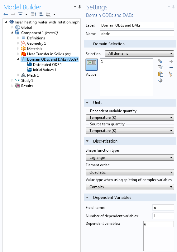
The Domain ODEs and DAEs interface for tracking the solution at the previous time step.
The screenshot above shows the relevant settings for the Domain ODEs and DAEs interface. Note that the units of both the dependent variable and the source are set to Temperature. It is a good modeling practice to appropriately set units. The discretization is set to a Lagrange Quadratic, which matches the discretization used by the Heat Transfer in Solids interface. You will always want to make sure that you are using the appropriate discretization. The name of the field variable here is left at the default “u”, although you can rename it to anything you would like.
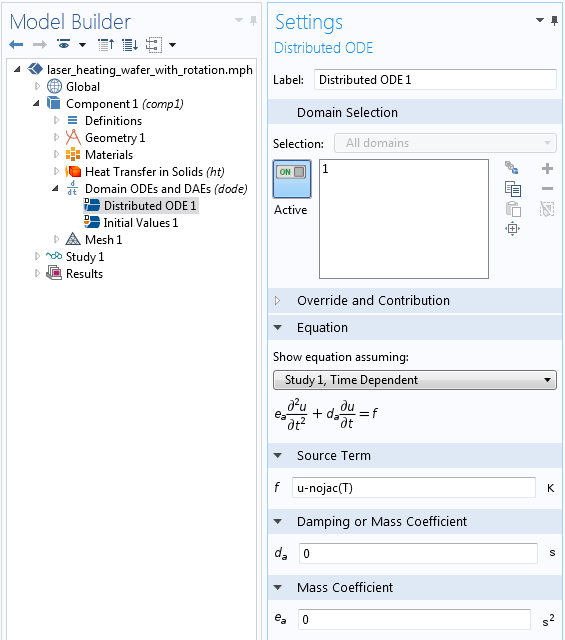
The equation being solved by the Domain ODEs and DAEs interface.
The screenshot above shows the equation that stores the temperature solution at the previous time step. This equation can be read as:
u-nojac(T)=0
The nojac() operator is needed, since we do not want this equation to contribute to the Jacobian (the system matrix). Lastly, we need to specify that this equation should be evaluated at the previous time step. This is done within the Solver Configurations.
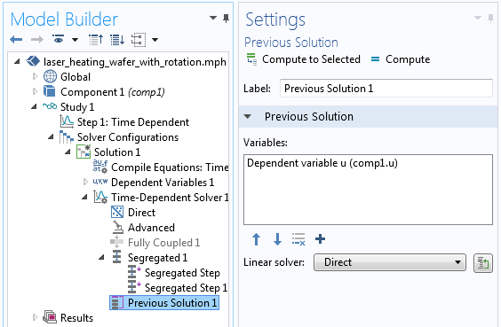
The Previous Solution feature added to the Solver Configuration.
The screenshot above shows the Previous Solution feature added to the Time-Dependent Solver. Once you add this feature, simply select the appropriate field variable to be evaluated at the previous time step. It will also be faster (although not necessary) to use the Segregated Solver rather than the Fully Coupled solver.
And that is all there is to it. You can now solve the model just as you usually do and you will be able to evaluate the temperature at the previous computational time step.
A More Practical Example: Keeping Track of the Maximum Temperature
Of course, having the solution at the previous time step isn’t really all that interesting in itself, but we can do quite a bit more than just store this solution. For example, we can apply logical expressions directly with the ODEs and DAEs equation interface. Consider the equation:
u-nojac(if(T>u,T,u))
This equation can be read as: “If the temperature at the previous time step is greater than u, set u equal to temperature. Otherwise, leave u unchanged.”
That is, it stores the maximum temperature reached at the previous time step at every point in the modeling domain. You can now evaluate the variables T and u at any point in the model to get both the temperature over time and the maximum temperature attained. To get the maximum temperature, you will want to take the maximum of the temperature at the previous time step and the temperature at the current time step, so you can introduce a variable in the model:
MaxTemp = max(T,u)
This will return the maximum temperature up to that time as shown in the plot below.
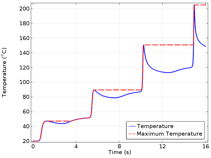
Temperature at a point plotted over time. The variable MaxTemp is also plotted and shows the maximum temperature reached up to that instant in time.
Summary
We have shown here the implementation of the newly introduced Previous Solution operator for time-dependent models. The three steps to use this functionality appropriately are:
- Choose the appropriate ODEs and DAEs interface and discretization.
- Enter an appropriate equation.
- Add the Previous Solution feature to the Solver Configurations.
We have shown how to evaluate the maximum temperature in this example, but there is a great deal more that can be done with this functionality, so stay tuned!


Comments (22)
Gongda Lu
July 11, 2015Gongda Lu
July 11, 2015Hello Walter,
Thanks a lot for sharing this new feature of COMSOL 5.1! Actually I have been longing for this functionality since a couple of years ago. Although it is a bit too late for me to implement that feature in my model, it does make a huge difference in the post-processing.
While I was practicing this functionality according to the example you provided, I was struggled by a problem: No data is stored after calculation, thus I can do nothing in the post-processing interface. However, the model does seem to have been executed properly because the “plot while solving” has presented the correct results I expected.
I am wondering if there is any other manipulation should be made in order to use the Previous Solution feature.
Your help is very much appreciated.
Best regards,
Gongda Lu
Walter Frei
July 13, 2015 COMSOL EmployeeDear Gongda,
This question will be best addressed via support, if you can please also send us the file you are having questions about.
Akash Aggarwal
August 24, 2015Hello Walter .
Is this can be done in COMSOL 5.0
With regards,
Akash Aggarwal
Walter Frei
August 24, 2015 COMSOL EmployeeHello Akash,
We do recommend that you always upgrade to the latest version of the software, the functionality being described here is new.
Anu Das
October 4, 2015Hello Walter
I was trying to couple poisson’s eqn (using electrostatics) and charge continuity eqn (using transport of diluted species) to study streamer discharge phenomena. I used the BC properly. they worked fine while run independently but coupling them didn’t converge. I tried it number of times but hardly any progress. So please send me your suggestions.
Regards,
– Anu Das
Anu Das
October 5, 2015I have prepared the ppt slides (4 nos.) showing briefly the steps i followed in comsol and trying to solve. I want to share this with you so plz let me know your email.
Regards
– Anu Das
Julien Givernaud
February 19, 2016This new feature can be very helpfull to implement very simple hysteresis loop over material properties
Best regards,
Julien
Walter Frei
April 13, 2017 COMSOL EmployeeIn followup to Julien’s comment about hysteresis modeling, please see:
https://www.comsol.com/blogs/thermal-modeling-of-phase-change-materials-with-hysteresis/
Saad Pasha
April 20, 2017Hi,
I’m totally unable to solve an ODE by using Domain-ODE module 🙁 The equation is:
dNp/dt = 10e9*exp((Vm/0.245)^2)*(1-(Np/(1.5e9*exp(2.46(Vm/0.245)^2))))
where ‘Vm’ is a field variable and may be assumed as:
Vm = ec.normE/maximumOf(ec.normE)
i.e. 0 <= Vm <= 1
and
ec.normE is electric field computed by Electrical Currents(ec) Module on the below 2D 48x48mm model with 300V applied pulse of 0.1s at 0.5mm electrode in 5 second simulation.
___________
| |
| o o |
| |
'————'
Kindly help me out and make me the model if possible. I'll be very thankful to you 🙁
Caty Fairclough
May 5, 2017Hi Saad,
Thanks for your comment and interest in this blog post!
For questions related to your modeling, please contact our Support team.
Online Support Center: https://www.comsol.com/support
Email: support@comsol.com
Walter Frei
May 8, 2017 COMSOL EmployeeHello,
We should also say that the timemax and timemin operators within more recent versions of the software do make this example of monitoring peak temperature somewhat moot. However, for some more relevant examples of using the previous solution operator, please see:
https://www.comsol.com/blogs/tracking-material-damage-with-the-previous-solution-operator/
https://www.comsol.com/blogs/thermal-modeling-of-phase-change-materials-with-hysteresis/
Dejan Krizaj
November 28, 2018Dear Walter,
In my model am trying to set a global variable y(t) where the current value is dependent on the previous one i.e. y(t)=y(t-1)+”some term on t”
Note: (t) and (t-1) used here are just notations of current and previous steps.
But before doing that, for the start, I just wanted to establish a proper evaluation of y at current and previous steps.
Therefore, I have defined y(t) = t[1/s]+1 as a global variable and followed the process described in this post:
1. Adding Global ODEs and DEA,
2. Defining u-nojac(y) with an initial value equal to 0.
3. Adding a Previous solution feature in the time-dependent solver.
So, this is working fine but with one small problem.
When I use Global evaluation in postprocesing, instead of getting
u = y (t-1)
i get u = y(t-1)+ “some error”.
“some error” is not constant and it is biggest at the start of the simulation and drops to 0 after some number of time steps.
What could be a reason for this?
Since both y and u are global variables analytically defined I presume they should not be dependent on some solver error or similar.
Best, Dejan
Jing Yuan
January 28, 2019Dear Walter,
Thanks a lot for posting this instruction. I’m working on a time dependent heat transfer problem, the boundary condition needs to be updated at each time step. could you give me any suggestion on it?
For example, for the boundary condition, the heat transfer coefficient h depends on a variable P, which should be calculated from last time step.
P=z2-0.1*z1, (Global ODE and DAE)
where z2=z1+2*integral(heat flux along a wall) (Boundary ODEs and DAEs)
I have to calculate z2 at each time step, then make z1=z2, so that I can use this value for next time step.
How can I make z1=z2 and not affect when I do z2=z1+(……)?
could you please give me some suggestion? Do you think it’s even possible to make it work with Comsol?
John Lionel
April 5, 2021Hi Walter,
Thanks a lot for the post! I have a question about the variable MaxTemp. From the equation u-nojac(if(T>u,T,u)), it seems that u has already stored the maximum temperature at every point. So why do we need MaxTemp? If we plot u at a certain point, we should get the same figure as the one plotted using MaxTemp. Thank you again for your post!
John
Walter Frei
April 6, 2021 COMSOL EmployeeHi John,
Not quite, as u is the maximum of the temperature at the previous timestep, so T can be greater than u.
Also, this post is quite old, see also:
https://www.comsol.com/blogs/how-to-use-state-variables-in-comsol-multiphysics/
As well as the timemax, timemin, attimemax, & attimemin operators.
Emil Rasmussen
April 26, 2021Is it possible to use this feature, to set the boundary temperature of a domain to the boundary temperature evaluated at previous time step of a different domain?
E.g. after 60 seconds, set the boundary temperature of the top boundary to the boundary temperature evaluated at the bottom of the domain and vice versa?
Walter Frei
April 26, 2021 COMSOL EmployeeHello Emil,
For what you are describing, you may also want to look to the Events interface, with reinitialization. See, as a starting point:
https://www.comsol.com/support/knowledgebase/1245
Songcai Han
August 20, 2021It works well for homogeneous materials. However, it is found that the solutions at previous step cannot be accurately recorded for a model with heterogeneous material properties, no matter what shape function you set in ODE. Why?
展昀 鄭
May 6, 2024Hello Walter,
I am a graduate student of National Chung Cheng University in Taiwan.
Thank you for sharing, but I still have some questions about the model that I would like to ask you. Can you give me your email or contact me via email?
Email: joker10530132@gmail.com
Best regards,
ZhanYun Zheng
Amin Kazemi
May 16, 2024Hi Walter,
Is it possible to utilize the solution from a previous iteration in the segregated solver for stationary studies?
Amin
Walter Frei
May 17, 2024 COMSOL EmployeeHello Amin,
You could, but you may also want to investigate state variables: https://www.comsol.com/blogs/how-to-use-state-variables-in-comsol-multiphysics/