
What do heated soap bubbles, wavy clouds, and Jupiter’s Great Red Spot have in common? Their formation depends on the dynamics of the shear layer existing between two parallel streams moving at different velocities. This unstable motion, called Kelvin-Helmholtz instability, is ubiquitous and plays an important role in the dynamics of climate, for example. Let’s take a closer look at the onset and evolution of this instability with the help of Computational Fluid Dynamics (CFD) analysis.
Heated Soap Bubbles
I recently read a NewScientist article, “Soap-bubble cyclone is a deadly storm in miniature”, where a group of physicists at the University of Bordeaux, France heated soap bubbles from underneath to create spinning storm-like structures. The resulting patterns resembled tropical cyclones in earth’s atmosphere, and it got me thinking of how to model this using COMSOL Multiphysics.
But first, let’s go over the concept of a shear layer.
What Is a Shear Layer?
A shear layer is a region of finite thickness with steep velocity gradients separating two parallel streams in contact and moving at different speeds. For the Kelvin-Helmholtz instability, small perturbations of the shear layer trigger its evolution into an array of large-scale vortices dissipating into smaller ones.
Easier visualized than explained in words, let’s take a look at two natural phenomena.
Wavy Clouds
In the figure below, you can see a rolling wavy cloud, also known as billow. The stream above the cloud is moving towards the right, while the cloud can be either still or moving towards the left. A small perturbation in their separation plane, i.e. the shear layer, triggers the rolling motion that gives these clouds their characteristic shape, which indicates a region of high turbulence that aircraft should avoid.
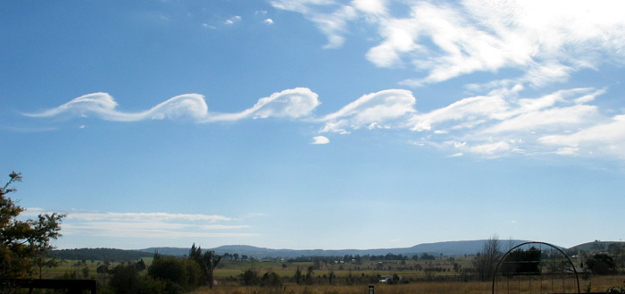
Rolling wavy cloud caused by the Kelvin-Helmholtz instability. Photo credit: GRAHAMUK.
Jupiter’s Great Red Spot
Jupiter’s Great Red Spot, shown below, was developed between 150 and 300 years ago, is about 2-3 times the size of earth, and is the fiercest manifestation of the Kelvin-Helmholtz instability in our solar system. At least four shear layers can be seen in this image, with the Great Red Spot being the biggest roll trapped between two jet streams.
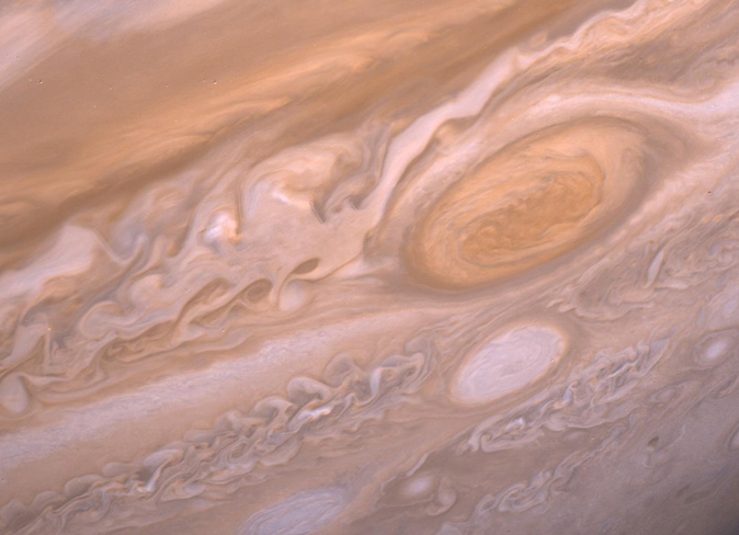
Image taken by a Voyager 2 flyby showing Jupiter’s storms in the neighborhood of the Great Red Spot. Photo credit: National Aeronautics and Space Administration (NASA).
Modeling the Dynamics of a Jet
The Kelvin-Helmholtz instability can be found everywhere in nature and can be used industrially, such as to enhance mixing applications, for instance. When working to predict or prevent the onset of the Kelvin-Helmholtz instability, simulation can be of great help to designers.
In order to trigger the Kelvin-Helmholtz instability, we need to define an initial velocity field consisting of a finitely thick, horizontally aligned shear layer with a vertical velocity perturbation. To simulate a jet with COMSOL Multiphysics, we can use the values from the article “A Second-Order Projection Method for the Incompressible Navier Stokes Equations”.
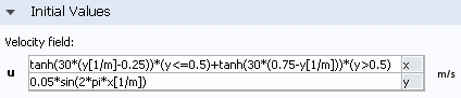
We want to use the following expressions for the initial velocity field:
u_{0} = \{ \begin{array}{l l} \tanh(30(y-0.25)) & \text{if} \quad y \leq 0.5 \\ \tanh(30(0.75-y)) & \text{if} \quad y > 0.5 \end{array}
v_{0} = 0.05 \sin(2 \pi x)
If we type these expression into the Initial Values settings window in the COMSOL software:
we can visualize the velocity field:
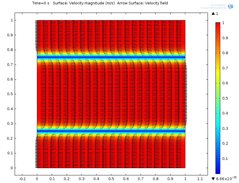
Velocity magnitude and arrow surface plot at t = 0 s.
In addition to the CFD analysis, we can also perform a mass transport simulation to try to mimic the results obtained from the work mentioned in the NewScientist article on soap-bubble cyclones.
We want to use the following initial concentration expression:
c_{0} = \{ \begin{array}{l l} (1 + \tanh(30(y-0.25)))/2 & \text{if} \quad y \leq 0.5 \\ (1 + \tanh(30(0.75-y)))/2 & \text{if} \quad y > 0.5 \end{array}
If we type this into the Initial Values settings window:
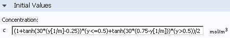
we can visualize the concentration:
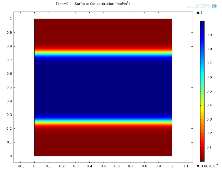
Concentration at t = 0 s.
The simulation is performed inside a unit square with Periodic Flow Conditions, so as to let the initial velocity field develop into a doubly periodic shear layer. To produce the above results, the density and viscosity should be set to 1 kg/m3 and 10-4 Pa·s, respectively. A similar Periodic Condition should be used for the mass transport simulation.
Taking a Closer Look at Shear Layers with Simulations
The simulation results show how the shear layers surrounding the central jet evolve into periodic vortices as shown in the animation below. Three rolls can be observed, two on top, rotating counterclockwise, and one below, rotating clockwise. The shear layers wrap around these rolls and are progressively thinned by the large straining field caused by the Kelvin-Helmholtz instability. Kinetic energy is transferred from the jet to the shear layers, which will continue to thin and dissipate into smaller vortices.
Animation of the CFD analysis results. Top-left plot: Pressure field. Top-right plot: Velocity magnitude and Arrow Surface. Bottom-left plot: Vorticity surface, vorticity contours, and velocity Arrow Surface. Bottom-right plot: Arrow Line. Left legend: Vorticity [1/a]. Top-right legend: Pressure [Pa]. Bottom-right legend: Velocity magnitude [m/s].
Given the symmetry of the initial values and the boundary conditions we used, the evolution of the top and bottom layers are mirrored. Below, you can see the results at t = 2 s. The high-frequency components of the vorticity field are smeared because the mesh is not fine enough to resolve the details of the flow.
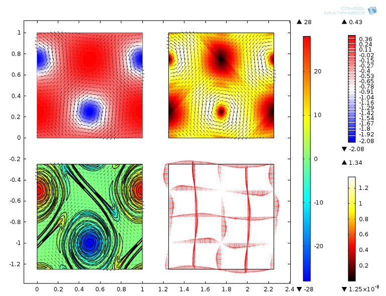
CFD analysis results at t = 2 s.
In order to overcome such limitations, a finer mesh is needed, which will result in higher memory demand and longer computational time — both of which are outside the scope of this blog post. Nevertheless, in this simulation, the larger vortices don’t exhibit oscillations or shape distortions, which indicates a good resolution of the overall dynamic behavior of the jet. Their onset is characteristically slow until a point is reached when the instability develops quickly and fully.
In the mass transport simulation, we consider the concentration to diffuse and be passively advected by the jet. In the simulation results below, you can notice that the dynamics of the concentration tightly follow the jet evolution even in the presence of the diffusion mechanism. The simulation results resemble the phenomena discussed in the NewScientist soap bubble article.
Mass transport simulation animation. Legend: Concentration [mol/m3].
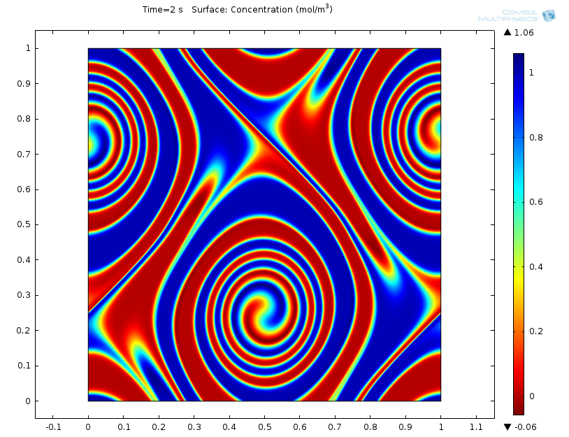
Mass transport simulation results at t = 2 s.
When studying the dynamics of a physical phenomenon with simulation, postprocessing is of paramount importance since it can confirm a physical intuition, give us better insight into what we’re studying, or show unexpected behavior. In this case, we can expect dust or ice crystals to be trapped within the rolls.
Here, I used the Particle Tracing Module to simulate such a scenario. The animation and particle trajectories plot confirm what we intuitively expected.
Particle tracing simulation animation.
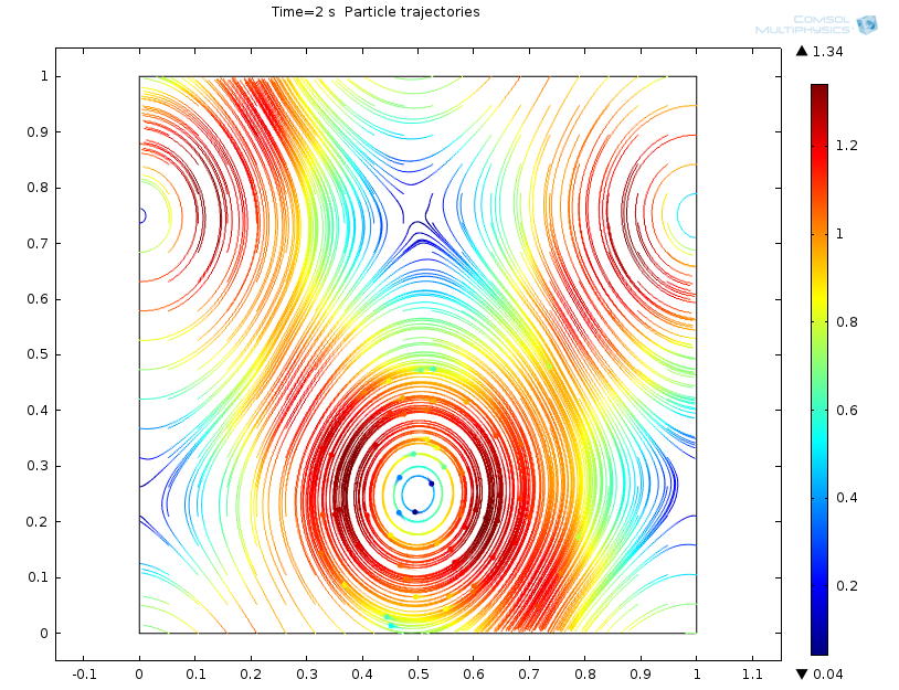
Particle tracing results at t = 2 s.
The next step could be the determination of residence time, which, if the Great Red Spot is concerned, might range from 150 to 300 years.


Comments (2)
Gertjan van Zwieten
December 13, 2014Hi Valerio, thanks a lot for the clear model description. For a course on turbulence I aim to set up a small tutorial simulating some vortex structures like this one, but I am running into problems relating to the periodic domain, as described in this [1] forum post. Seeing that you didn’t have these issues, would you perhaps weigh in on this discussion and explain what extra step I am overlooking to make this type of simulation work? Much appreciated!
[1] http://www.comsol.nl/community/forums/general/thread/54451/
Valerio Marra
December 23, 2014Hi Gertjan,
I was reading the thread and it looks like your fellow COMSOL users helped you out successfully.
Let me know if you need anything else and as usual, please contact support@comsol.com if you have any technical questions.
Best regards,
Valerio