
Electrochemical impedance spectroscopy (EIS) is widely used for studying electrochemical systems. It reveals key electrochemical processes like charge transfer, mass transport, and surface effects. This blog post demonstrates how to model nonideal behaviors like adsorption, diffusion limits, and surface roughness in the COMSOL Multiphysics® software — beyond traditional equivalent circuits. You’ll also learn how to implement the local constant phase element (CPE) when its underlying mechanism is unclear.
Practical Applications of Electrochemical Impedance Spectroscopy
Many electrochemical systems involve multiple overlapping processes, which can make it challenging to pinpoint the factors that affect performance. By applying a small sinusoidal signal across an electrochemical system and measuring its response over a range of frequencies, EIS provides a window into the intricate processes of charge transfer, mass transport, and double-layer effects: key phenomena that dictate the performance of the system. Due to its high sensitivity to small current changes, EIS can detect minor variations that might otherwise remain unnoticed.
The benefits are clear when looking at real-world electrochemical systems:
- Batteries: From consumer electronics to electric vehicles, EIS can be used to analyze ion and electron transport within the cell, identifying potential degradation and capacity fade.
- Corrosion: Early signs of corrosion in pipelines, marine structures, and concrete reinforcements can be detected by EIS through the tracking of changes at metal–electrolyte interfaces over time.
- Fuel cells: Catalyst layers, membranes, and reactant flows can be evaluated using EIS, providing insights that contribute to improved fuel cell performance and longevity.
- Sensors: Electrode interactions with target molecules can be assessed by EIS, enabling applications such as glucose monitoring through the detection of concentration changes in biological fluids.
Examples of electrochemical systems using EIS can be viewed in the slideshow below.
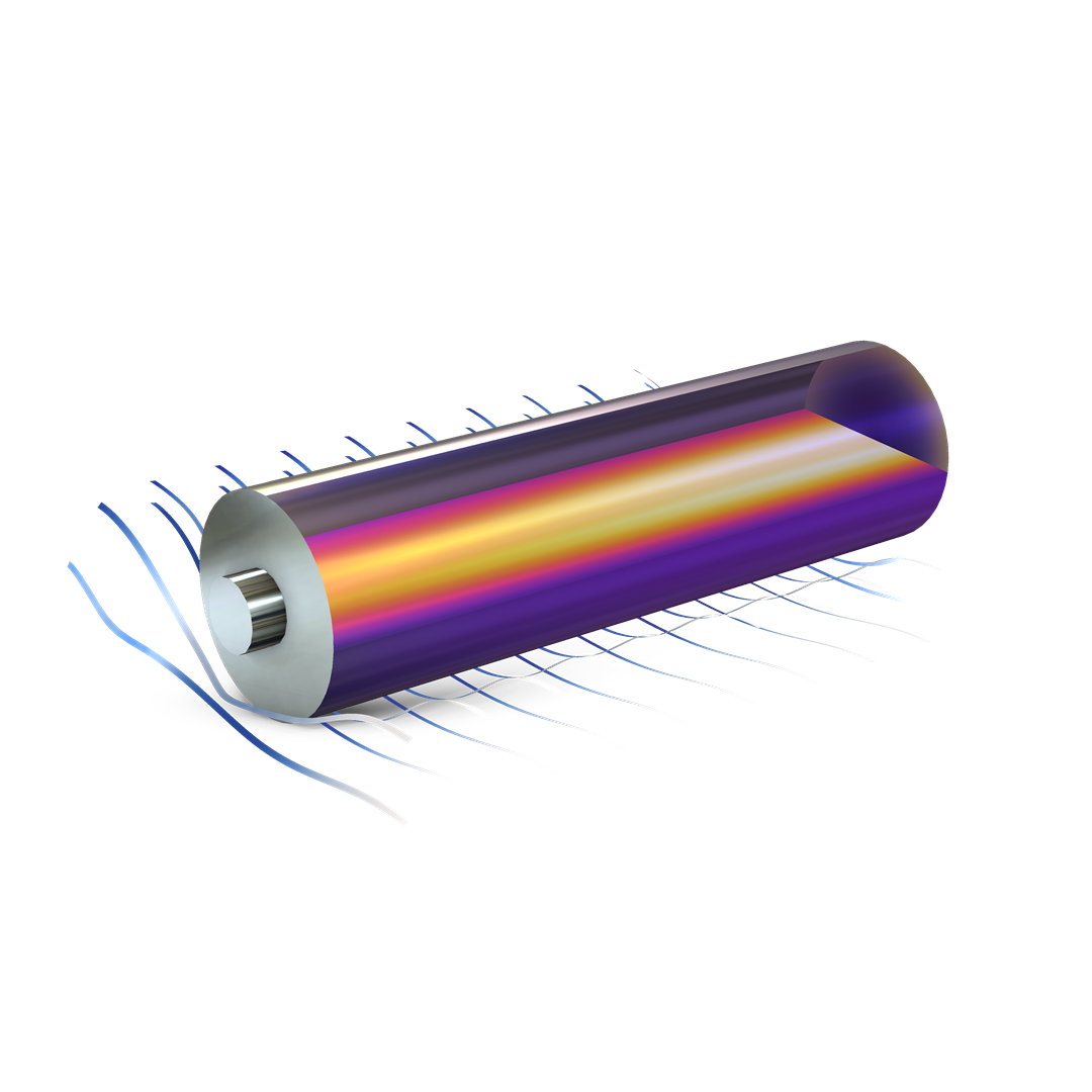 Lithium-ion batteries.
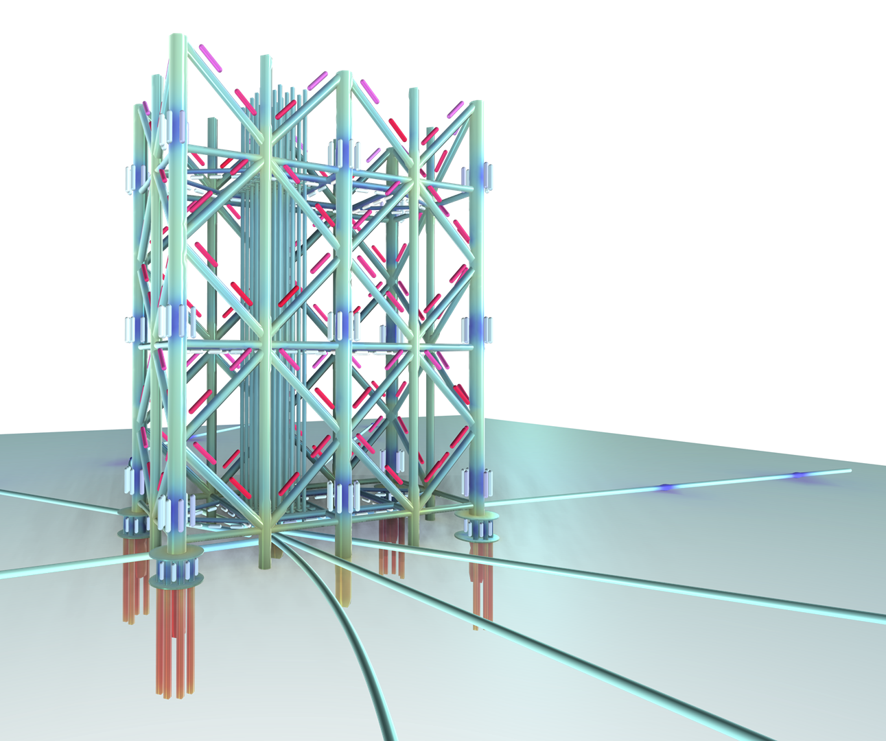 Offshore oil platforms.
 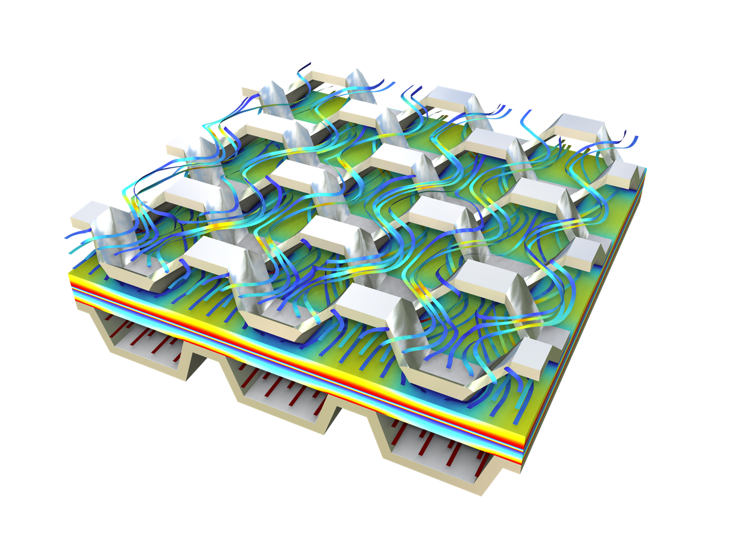 PEM fuel cells.
 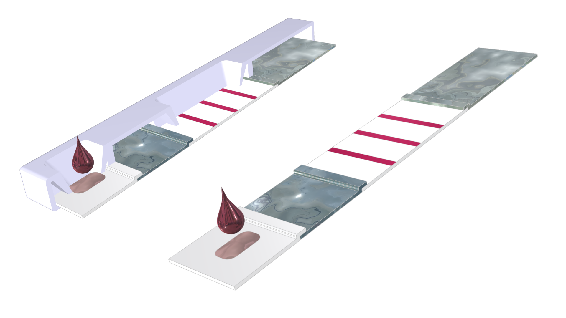 Rapid lateral flow assay tests.


Methods Beyond Equivalent Circuits
For a system undergoing a simple electrochemical reaction without considering mass transfer effects, the associated equivalent circuit can consist of a resistor in series with a parallel combination of a resistor and a capacitor. When presented in a Nyquist plot, it’s shown as a semicircle, the diameter of which corresponds to the magnitude of the charge transfer resistance.
 Equivalent circuit model of a resistance in series with RC pair.
 Nyquist plot for an equivalent circuit model.
Traditional equivalent-circuit elements have long been used to model simple electrochemical systems and fit the results to experimental data. However, the underlying coupled physical processes cannot be captured. Instead of relying solely on passive equivalent-circuit elements, a physics-based approach can be used to model the underlying processes for a realistic representation of electrochemical systems. In COMSOL Multiphysics®, this is achieved by solving the fundamental equations that govern electrochemical phenomena.
By incorporating mass transport, charge transfer, and reaction kinetics into simulations, the complex interplay of nonideal behaviors affecting the impedance response can be captured. For example, diffusion limitations can be modeled using mass transport equations, while adsorption–desorption behaviors can be captured through kinetic expressions. Additionally, electrode surface roughness can be incorporated into the model by defining the detailed electrode surface geometry. These combined approaches provide a realistic representation of complex electrochemical behaviors.
These nonidealities will be discussed in more detail in the following section.
Charge Transfer Reactions with Absorption and Desorption
Many electrochemical reactions involve intermediates or ions that adsorb onto the electrode surface. Adsorption introduces another dynamic aspect to the electrode–electrolyte interface because the surface coverage of adsorbed species can vary with potential and time, adding additional time constants to the system. Adsorption effects can be captured by incorporating kinetic expressions into the electrochemical model. For example, in the model example of copper deposition in a through-hole via, two adsorbed species — chloride (Cl⁻) and a suppressor additive polyether (P) — are modeled using the Adsorbing-Desorbing Species feature defined at the Electrode Surface boundary condition.
These species may adsorb or desorb during faradaic or nonfaradaic reactions. Beyond the transient analysis originally performed, impedance responses are simulated using a separate frequency-domain perturbation study at two elapsed times (t = 0 min and t = 2 min). Initially, the surface coverage of the adsorbed species (P) is low, but at t = 2 min, coverage significantly increases and becomes nonuniform. The presence and distribution of adsorbed species significantly influences the impedance response, altering the impedance spectra from an initial two-capacitive-loop behavior at low surface coverage to a response exhibiting a pronounced low-frequency inductive loop at higher coverage. Impedance response can also vary when systems have adsorbed species, which will depends on system operating conditions and surface coverage (Ref. 1).
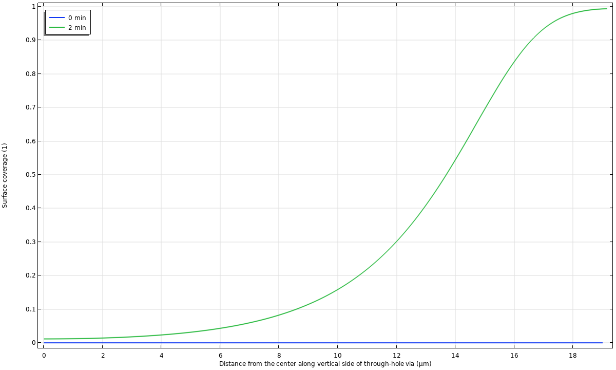 Surface coverage for adsorbed species on an electrode surface at two different elapsed times (t = 0 min and t = 2 min).
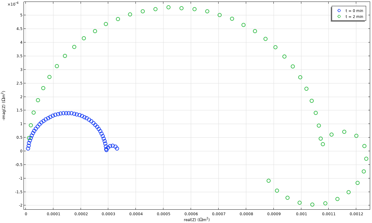 Nyquist plot of an electrochemical cell at two elapsed times (t = 0 min and t = 2 min).
Impact of Mass Transport
Mass transport in electrochemical systems can be modeled by solving governing equations. For example, in fuel cells, gas transport (e.g., hydrogen and oxygen) involves both diffusion and convection, influenced by properties of porous catalyst layers and gas diffusion layers (GDLs). These transport phenomena directly affect the impedance response. In the tutorial model of species transport in the gas diffusions layers of a PEM, species transport is modeled within the GDLs of a proton exchange membrane (PEM) fuel cell by coupling charge conservation; Maxwell–Stefan diffusion equations for reactants, water, and nitrogen; and Darcy’s law for gas flow. In the resulting polarization curve (shown in the figure below), as the cell voltage moves toward more cathodic values, the current density initially increases until reaching a plateau due to mass transport limitations.
In addition to the original example, an EIS study is performed to further distinguish contributions from reaction kinetics and mass transport at operating voltages of 0.4 V, 0 V, and -0.4 V. At a cell voltage of 0.4 V, the Nyquist plot shows two distinct loops: The high-frequency loop corresponds primarily to charge-transfer reactions while the low-frequency loop is related to gas diffusion processes in the GDL. At a more cathodic potentials of 0 V, merging impedance loops indicate overlapping time constants for reaction kinetics and diffusion. At an even lower potential of -0.4 V, impedance becomes dominated by diffusion, resulting in a single large loop as the system approaches mass transport limitations, while charge-transfer resistance becomes much smaller.
 Polarization curve for a PEM fuel cell.
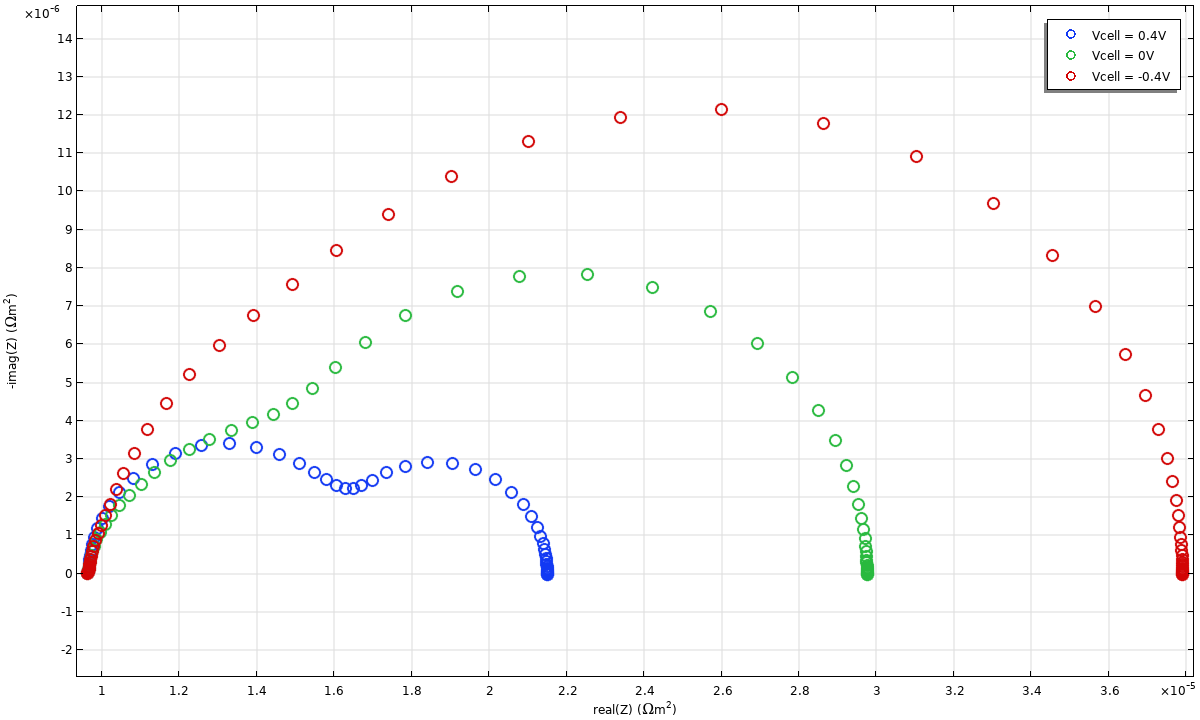 Nyquist plots of the PEM fuel cell at operating potentials of 0.4 V, 0 V, and -0.4 V.
Effects of Electrode Surface Roughness
Surface roughness introduces another nonideality in electrochemical systems, which can affect the impedance response. Variations in electrode surface structures, such as unevenness, porosity, and other inhomogeneities, can affect local current distribution. In COMSOL Multiphysics®, surface roughness can be explicitly incorporated through geometry modifications.
As illustrated in the figure below, two different electrode surfaces are modeled:
- Rough electrode represented by a Koch snowflake structure
- Smooth, flat electrode
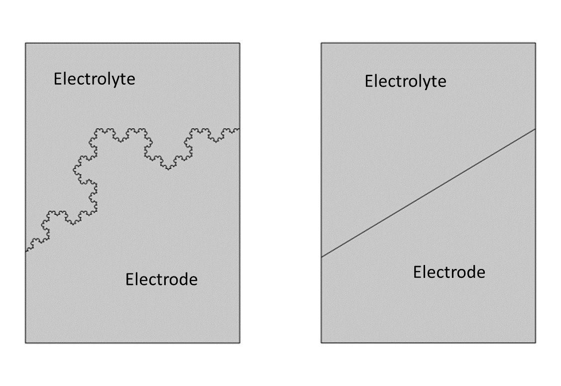 Geometry of a cell with different electrode surface shapes: a Koch snowflake and flat surface.
The impedance response can be analyzed using the secondary current distribution without considering mass transport. The dimensionless impedance responses, presented in Nyquist plots, shows distinct behaviors for the two surface configurations. A semicircle is observed for the flat electrode surface, while it shows high-frequency dispersion for the rough electrode. This dispersion can be attributed to frequency-dependent complex ohmic impedance (Ref. 2). Such impedance behavior can be seen above a characteristic frequency that depends on electrode roughness shape and size, electrode geometry, and electrolyte conductivity.
 Nyquist plot for the Koch snowflake and flat electrode surfaces.
Constant Phase Element
While physics-based modeling provides insights into many nonidealities, such as charge transfer reactions with adsorption and desorption, mass transport effects, and electrode surface roughness, there are scenarios where the observed impedance behavior cannot be fully explained by these known mechanisms. In some cases, a constant phase element (CPE) is normally used to improve the fit of models to the impedance data. Unlike an ideal capacitor, which has a phase angle of -90 degrees, a CPE has a phase angle that can vary between 0 and -90 degrees, depending on the characteristics of the electrochemical system.
 Electrical symbol for the constant phase element (CPE).
Mathematically, the impedance of a CPE can be defined as
where Q and α are CPE parameters, i is the imaginary number, ω is the angular frequency, and α is a parameter that ranges from 0 (a resistor) to 1 (an ideal capacitor).
Incorporating Local Constant Phase Elements on Electrode Reactions
In COMSOL Multiphysics®, local CPE behavior can be integrated into models through various electrochemistry-related physics settings. One common approach involves applying CPEs via boundary conditions under Porous Electrode or Electrode Surface, allowing for the specification of capacitance that represents interfacial effects.
The tutorial for modeling impedance in a lithium-ion battery studies the impedance of a full lithium-ion battery cell. Porous Matrix Double-Layer Capacitance is used to define the nonfaradaic double-layer current density at the interface between the porous electrode matrix and the electrolyte. When modeling pure capacitance, a constant value is normally assigned, ranging from 0.2 F/m² to 0.5 F/m² for electrical double-layer capacitance.
Capacitive (charging) current can be written as
where (\phi_{\mathrm{s}} – \phi_{\mathrm{l}} – \Delta \phi_{\mathrm{s,film}}) is the potential difference applied on the electrochemical reactions, including the effect of potential drop due to the presence of a film, and C_{\mathrm{dl}} is the electrical double layer capacitance.
 Modeling the constant phase element under a Porous Electrode node.
Instead of using a constant value for the pure capacitance, the expression to describe the electrical double layer capacitance needs to be modified to include the local CPE effect.
C_{\mathrm{dl} could be written as
which yields the capacitive current expression as
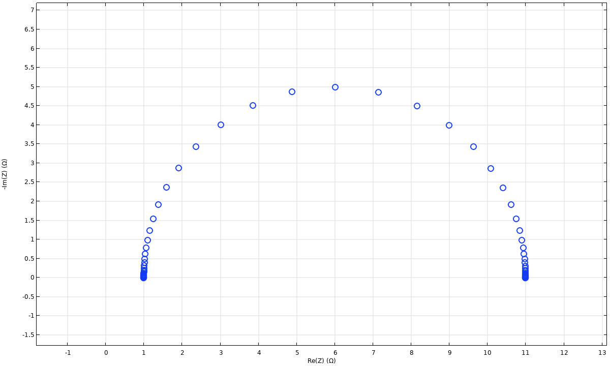
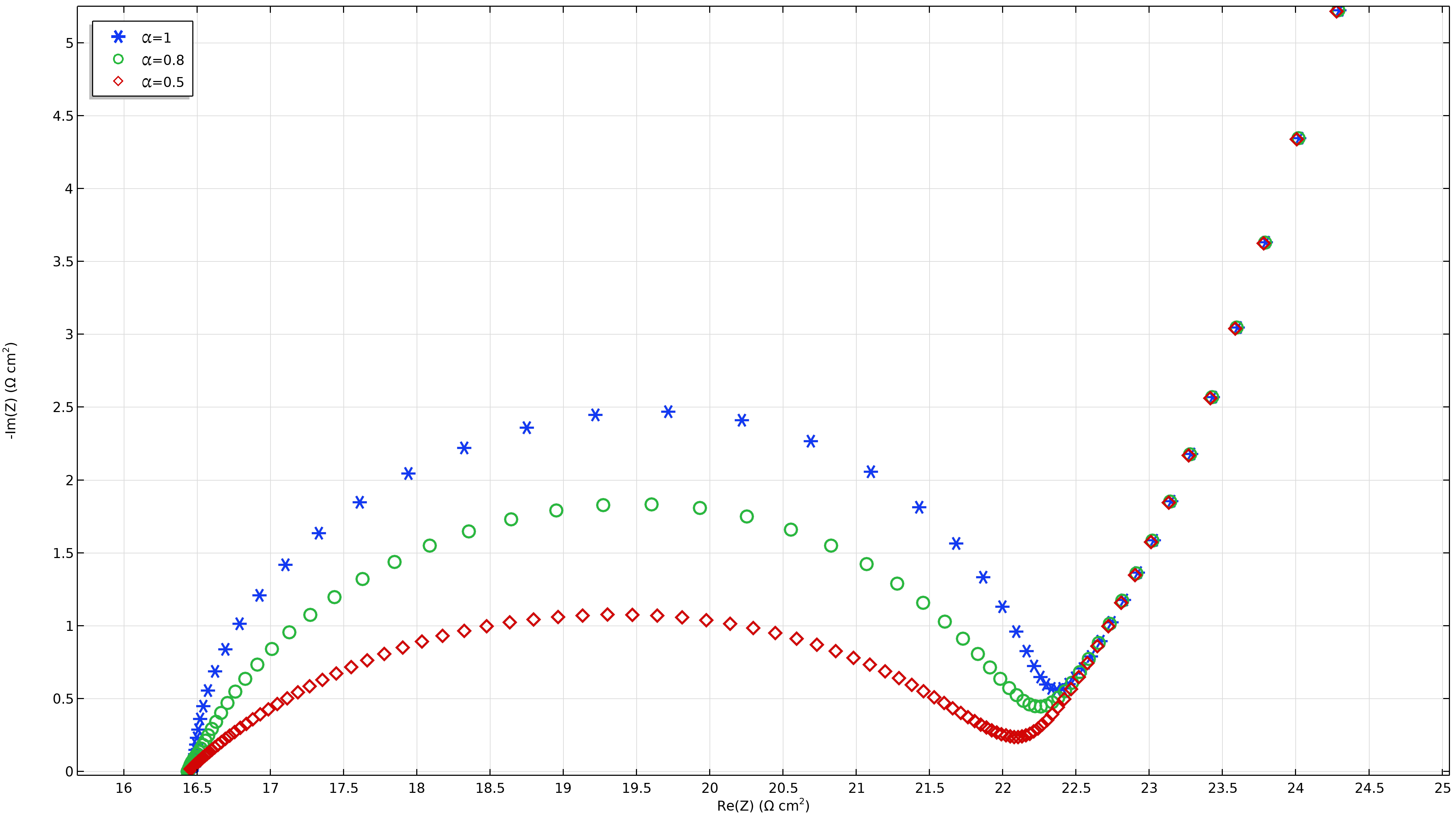 Nyquist plot with different values of alpha as a parameter.
As shown in the figure above, Nyquist plots show impedance for different values of alpha (1, 0.8, and 0.5), with the real part of impedance on the x-axis and the negative imaginary part on the y-axis. The plots exhibit a characteristic semicircular shape arc followed by a tail, representing charge transfer and diffusion processes. As alpha decreases, the semicircle becomes more depressed and shifts downward.
Although the exact origin of CPE behavior at metallic electrodes remains unresolved, CPE parameters are typically used to extract capacitance by assuming either a distribution of time constants across the electrode surface or the presence of a film. The values of alpha generally depend on system characteristics such as film presence, surface inhomogeneities, and mass transfer effects within porous electrodes (Ref. 3). Electrosorption-diffusion of anions was also suggested as another potential mechanism (Ref. 4).
CPE can also be modeled through equivalent circuits in COMSOL Multiphysics®, incorporating components such as resistors, capacitors, and inductors. A Resistor-Capacitor Couple is added, where the resistance R is set to a chosen value (e.g., 1 Ω), and the capacitance C follows the CPE formulation. This approach allows the circuit to approximate nonideal electrochemical behavior by adjusting CPE parameters.
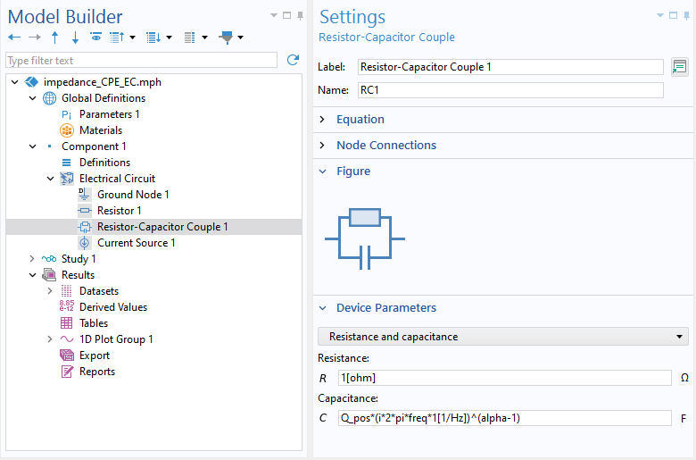 Modeling constant phase elements in an electrical circuit.
To ensure the model accurately reflects experimental impedance data, parameter estimation can be applied in COMSOL Multiphysics®. The CPE parameters, such as Q and α, can be defined as control variables and systematically optimized to fit measured experimental data. Parameter estimation, available in all electrochemistry-related add-on products, refines the model by minimizing discrepancies between simulated and experimental results. The example “Modeling Impedance in the Lithium-Ion Battery” demonstrates how the Parameter Estimation study step can be used to systematically adjust model parameters effectively. By iteratively refining the parameters, the simulation aligns closely with experimental observations.
Nonidealities in EIS
This blog post has explored the use of COMSOL Multiphysics® to model nonidealities in electrochemical impedance spectroscopy (EIS). By explicitly simulating phenomena such as adsorption-desorption kinetics, mass transport limitations, and electrode surface roughness, physics-based modeling provides insights beyond traditional equivalent circuit approaches.
Additionally, when impedance behaviors cannot be fully explained by known mechanisms, incorporating a local constant phase element can help represent these residual effects. Such modeling capabilities allow researchers to characterize and understand electrochemical systems across diverse use cases, including batteries, corrosion protection, fuel cells, and sensors.
References
- V. Vivier and M. E. Orazem, “Impedance Analysis of Electrochemical Systems,” Chemical Reviews, vol. 122, issue 12, article 11131–11168, 2022.
- C. You. et al., “Experimental observation of ohmic impedance,” Electrochimica Acta, vol. 413, 2022.
- S. Wang et al., “Electrochemical impedance spectroscopy,” Nature Reviews Methods Primers, vol. 1, article 41, 2021. Doi: 10.1038/s43586-021-00039-w
- A. Lasia, “The Origin of the Constant Phase Element,” J. Phys. Chem. Lett., vol. 13, issue 2, pp. 580–589, 2022.


Comments (0)