Previously on the blog, we introduced you to the tears of wine phenomenon and its cause — the Marangoni effect. This effect results from a gradient of surface tension at the interface between two phases. In situations where a surface gradient is temperature dependent, the Marangoni effect is referred to as Marangoni convection. Here, we will demonstrate how to analyze Marangoni convection in COMSOL Multiphysics and easily separate effects, such as gravity, in your simulations.
The Challenges of Studying Marangoni Convection
Marangoni convection — also called thermocapillary convection — is important in a number of processes, including welding, crystal growth, and electron beam melting. Due to the types of metals used and the extremely high temperatures involved, performing experiments to analyze Marangoni convection often proves to be rather challenging. The impact of gravity, which mixes up this convective effect with the Marangoni effect, also adds to the difficulty of studying this phenomenon.
At NASA, researchers analyzed Marangoni convection to see how mass and heat move within a fluid under microgravity conditions. Conducting the experiment in microgravity enabled the research team to create silicone oil columns much larger than those that could be studied on Earth, offering a more detailed look at the flow and instability within them. Additionally, suppressing the influence of gravity helped eliminate the possibility of gravity-induced deformation, thus enhancing the accuracy of their results.
With numerical experiments, it is very easy to separate effects that are simply impossible to remove in an experiment on Earth. Our Marangoni Effect tutorial uses a transparent liquid at ambient temperatures to find the velocity field induced through the Marangoni effect in a fluid with known thermo-physical properties. The transparency of the silicone oil makes it easy to implement and compare our simulation results with the microgravity experimental findings.
A Simulation Analysis
To begin, we must solve the Navier-Stokes equations to model the velocity field and pressure distribution in the fluid. Keep in mind that variations in temperature affect the velocity and cause a buoyancy force that needs to be represented in the equations. This can be done by using the Boussinesq approximation in the Navier-Stokes equations.
With the Laminar Flow interface, we can solve the momentum balance equations. To solve for heat transfer, we use the Heat Transfer in Fluids interface. Finally, we use the Non-Isothermal Flow multiphysics coupling to set the convective term in the heat equation and the Marangoni Effect multiphysics coupling to impose that the shear stress is proportional to the temperature gradient.
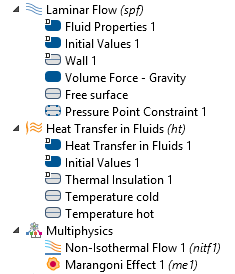
The setup of the tutorial model. The Multiphysics node contains both the nonisothermal coupling and the Marangoni effect.
This simulation presents three multiphysics couplings that must be solved using the nonlinear solver:
- Because of the temperature dependency of the fluid density, \rho, accounted for following the Boussinesq approximation, the gravity force, -\rho \textbf{g}, is given by an expression that includes temperature.
- Convective heat transfer depends on the velocity of the momentum balance.
- The Marangoni effect relates the shear stress applied at the free surface to the surface temperature gradient.
Simulation Results
In our simulations, we analyze a gradual increase in temperature difference between vertical walls. For an almost unnoticeable temperature increase of 1 mK, the temperature field and velocity field have only a slight relation, and the decrease appears linear from left to right.
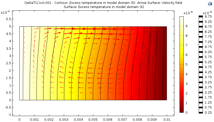
The results of a Marangoni effect simulation after only a small change in temperature. The background color represents the temperature field and the red arrows indicate the velocity field. The black lines are isotherms.
With an increase of 50 mK, Marangoni convection increases the fluid flow and temperature distribution. The temperature decrease is no longer linear across the plot.
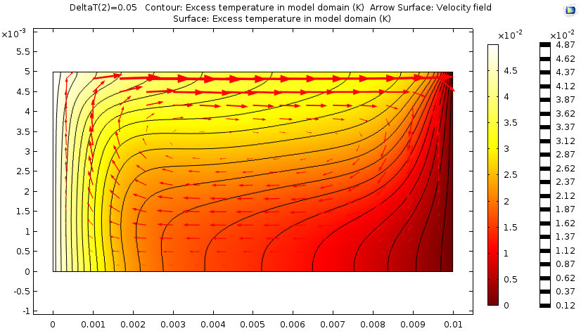
The results of the simulation after a temperature increase of 50 mK.
Finally, we test a temperature difference of 2 K. The temperature and velocity fields are distinctly coupled and the fluid accelerates at the surface where the temperature gradient is highest.
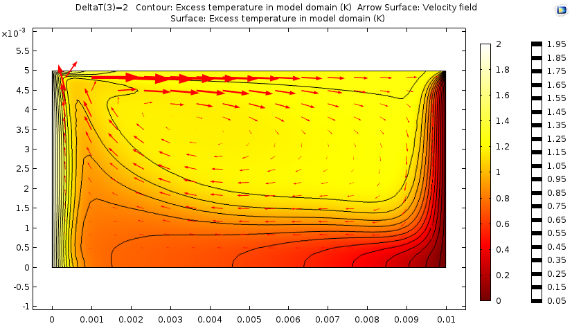
The results of the simulation when the temperature difference is raised to 2 K.
As indicated by the simulation results, the Marangoni effect becomes predominant as the difference in temperature increases.
Separating Gravity from the Marangoni Effect
For the same temperature difference of 2 K, we can easily remove the gravity contribution and keep the Marangoni effect. With the same objective of understanding how buoyancy forces compare with the Marangoni effect, we can simply disable the Marangoni contribution at the surface, leaving the surface free of stress. The results show that the Marangoni effect is predominant versus buoyancy forces. The shape of the curve shows a peak close to the cold right wall, which is characteristic of the fluid behavior of high Prandtl numbers.
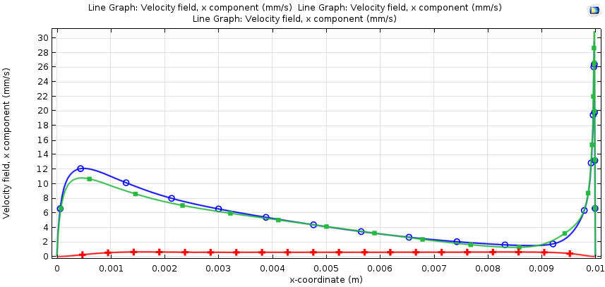
The results of the horizontal velocity at the surface versus the horizontal coordinate (m) for a temperature difference of 2 K. Blue represents both the Marangoni effect and the buoyancy effect; green represents only the Marangoni effect; and red represents only the buoyancy effect.
Summary
In this blog post, we have demonstrated how to set up a model representing an experiment combining gravity and Marangoni effects. Separating these two effects is challenging in an experimental setting. In numerical simulations, this process is straightforward, facilitating an understanding of each effect.
You can reproduce the results shown here by downloading the Marangoni Effect tutorial from our Application Gallery. This example uses the Non-Isothermal Flow and Marangoni Effect multiphysics couplings available in the Heat Transfer Module.
While we have focused our attention here on single-phase flows, it is worth mentioning that the Marangoni effect is also handled in the two-phase flow interfaces, which are available in the CFD Module and the Microfluidics Module.


Comments (10)
Omar Al-Rawi
April 5, 2017Dear Eric,
Thank you for this amazing blog.
If I want to model the Laminar Flow, Heat Transfer and Transport of Diluted Species interfaces together, dose the above process stay same in my model or I have to add another multiphysics node? What I am attempting to do is modelling the evaporation of sessile droplet under non-isothermal system.
Could you please clarify this situation?
Thanks,
Omar
Eric Favre
April 5, 2017 COMSOL EmployeeDear Omar,
Before answering, another important parameter could be if evaporation rate is large or not : depending on the answer, you can neglect the volume variation, or not! You can find details of the equations used when evaporation rate is small in Nancy’s blog here :
https://www.comsol.fr/blogs/intro-to-modeling-evaporative-cooling/
The next step of adding the volume decrease wrt the time is feasible by adding a moving mesh or ALE equation to your system and solving the exact same set of physics on the moving geometry.
Now to answer your question, if you don’t need to compute the volume variation, Marangoni flow should not prevent you from doing what you describe. If you want to take into account volume variations, then you probably need to add a moving mesh equation to control the shape of your droplet.
Good luck,
Eric Favre – COMSOL France Grenoble
Omar Al-Rawi
April 10, 2017Dear Eric,
Many thanks for your replying.
Actually, I have already taken into account the volume variation so that I have added the moving mesh equation to the system. What I am trying to ask is about the mutliphysics node. In your model, you added the Non-Isothermal Flow and Marangoni Effects nodes to couple the flow and heat transfer modules together. In my model, I am trying to compute the diffusion-convection physics in the air domain surrounding the evaporating droplet and thermal convection in side the droplet. So, are the above multiphysics nodes enough to couple all these physics (Laminar Flow, Heat Transfer and Transport of Diluted Species) or I need to add the Temperature Coupling to couple the heat transfer and transport of diluted species together?
Thanks,
Omar
Eric Favre
April 10, 2017 COMSOL EmployeeI guess so, although this is hard to be sure without a closer look at your problem and what hypothesis you consider to solve the problem you describe. If you want to make sure that what you have entered in COMSOL Multiphysics matches the equations of the problem you want to describe, I encourage you to send _both_ to tech support.
Best regards,
Eric
Phong Huynh
August 21, 2017Thank you very much for your post. I have try to reproduce your work. I have an error when building mesh as following:
Failed to insert point.
– x-coordinate: 9.83463
– y-coordinate: 5
A degenerated triangle was created.
I use Comsol 5.2
Could you help to figure out?
Thanks once more
Eric Favre
August 21, 2017 COMSOL EmployeeDear Phong Huynh,
that sounds strange that you get a mesh error in this simple rectangle geometry, whatever the version you use. I encourage you to send your file or details to technical support (https://www.comsol.com/support) to get help. The source file that contains the solved example together with the mesh can be found here : https://www.comsol.com/model/marangoni-effect-20329
Best regards,
Eric Favre
Phong Huynh
August 23, 2017Thanks very much. I made it.
Eric
February 22, 2019Greetings Eric,
I came cross your work on the modeling of an electrostatic precipitator (i.e. the fully coupled approach of modeling the electric potential and space charge density). I was able to obtain the solutions with precision (Thanks!) as compared to theoretical results for an axisymmetric domain.
More recently, as I merged a second domain on top of my first domain to study the entrance effect, I went into issues of getting converged solutions. I was wondering if you are interested in taking a look at my current model and maybe offer your suggestion in fixing the issues I am facing.
Thank you.
Eric
Eric Favre
February 23, 2019 COMSOL EmployeeHello Eric Monsu Lee,
I encourage you to contact the technical support directly with some details (comsol.com/support).
Thank you,
Eric Favre
Runjia Wang
October 13, 2025Dear Eric,
I noticed that this is uses the full Navier-Stokes equation, but a lot of times, the Marangoni effect can be manifested as the thin-film equation. Could I ask how to simulate it this way? Thanks.