Detailed modeling of the complex interaction of flow and acoustics is achieved in the COMSOL Multiphysics® software and add-on Acoustics Module using the linearized Navier-Stokes interfaces. With the release of version 5.3, the capabilities were further extended with the addition of a new stabilization scheme. This allows robust simulations of systems with acoustic properties that are modified by or depend on a turbulent background flow; e.g., automotive exhaust systems. Here, we introduce important modeling concepts and present application examples.
Introduction to Aeroacoustics Modeling
The complex interaction of a stationary background flow and an acoustic field can be modeled using the linearized Navier-Stokes physics interfaces in the Acoustics Module. The interfaces allow for a detailed analysis of how a flow, which can be both turbulent and nonisothermal, influences the acoustic field in different systems. This includes all linear effects in which a background flow interacts with and modifies an acoustic field. The linearized Navier-Stokes interfaces do not induce flow-induced noise source terms. Basically, the equations solve for the full linear perturbation to the general equations of CFD — mass, momentum, and energy conservation.
Being able to model and simulate the details of how a background flow influences an acoustic field is important in many industries and areas of application. In the automotive industry, the acoustic properties of exhaust and intake systems are altered when a flow passes through them. For example, the transmission loss of a muffler changes depending on the magnitude of the bypass background flow. In aerospace applications, the study of how liners and perforates behave acoustically when a flow is present is of high interest. The detailed acoustic properties (absorption, impedance, and reflection coefficients) of these subsystems influence the system-level behavior of, for example, a jet engine.
In the muffler and liner examples, the attenuation of the acoustic signal by the turbulence present in the background flow can also be captured with the linearized Navier-Stokes equations. Moreover, the background flows in these models are often nonisothermal in nature.
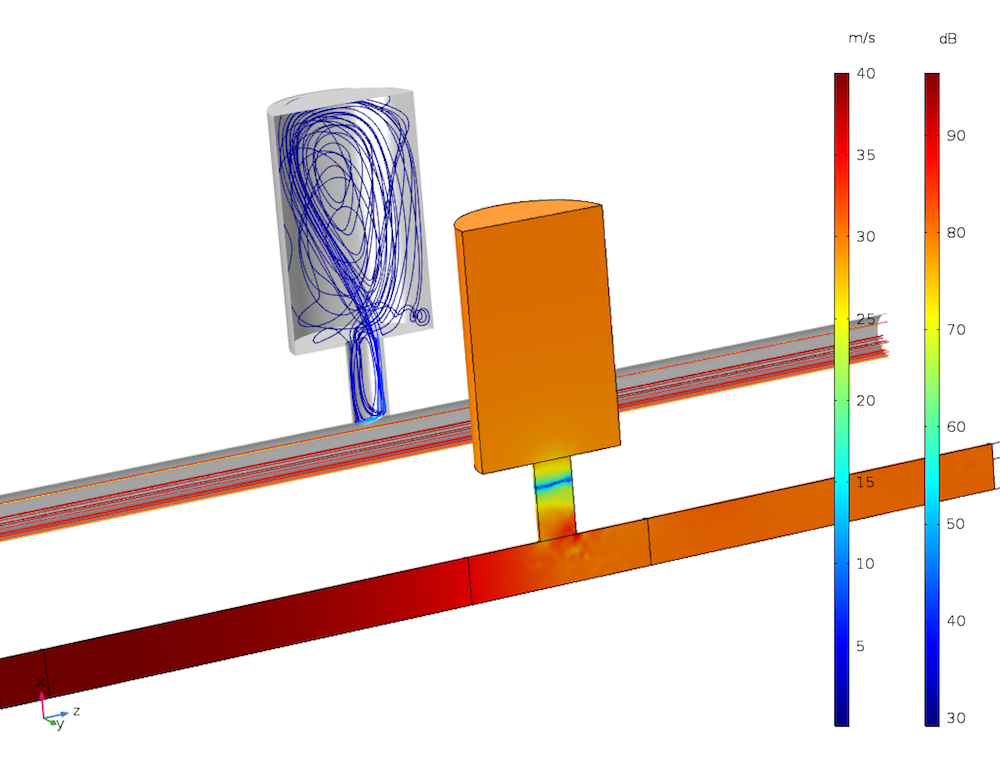
Example of an automotive application. Results from the Helmholtz resonator with flow example presented below. In front, the color surface plot is of the sound pressure level. At the back, the streamlines are of the background flow.
The linearized Navier-Stokes interfaces have a built-in multiphysics coupling to structures. This enables an out-of-the-box setup of fluid-structure interaction (FSI) models in the frequency domain (or in the linear regime in the time domain). The interaction of flow, acoustics, and structural vibrations is important in many applications. One application example is for flow sensing in a Coriolis flow meter. In general, these interfaces are suited for the analysis of the changed vibrational behavior of structures when under a fluid load caused by a background flow.
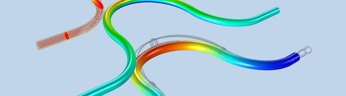
Example of FSI in the frequency domain: the movement of a Coriolis flow meter actuated at the fundamental frequency. The surface shows the structural deformation (the phase and amplitude are highly exaggerated for visualization) and the open cut-out section of the pipe shows the acoustic pressure on the pipe’s inner surface.
Other applications of the linearized Navier-Stokes interfaces include the study of combustion instabilities and general in-duct acoustics as well as more academic applications like analyzing the onset of flow instabilities or studying regions prone to whistling.
The interfaces now include the Galerkin least squares (GLS) stabilization scheme, enabling more robust simulations. This new default setting better handles the numerical and physical instabilities introduced by the convective and reactive terms included in the governing equations. Moreover, the reformulated slip boundary condition is now well suited when solving models with an iterative solver. This is crucial in cases where large industrial problems have to be solved.
The Linearized Navier-Stokes Equations
The linearized Navier-Stokes equations represent a linearization to the full set of governing equations for a compressible, viscous, and nonisothermal flow (the Navier-Stokes equations). It is performed as a first-order perturbation around the steady-state background flow defined by its pressure, velocity, temperature, and density (p0, u0, T0, and ρ0). This results in the governing equations for the propagation of small perturbations in the pressure, velocity, and temperature (p, u, and T) — the dependent variables. In perturbation theory, a subscript 1 is sometimes used to express that these variables are first-order perturbations. The governing equations (with subscript 0 on the background fields) read:
(1)
& \frac{\partial \rho}{\partial t}+\nabla\cdot(\rho_0 \mathbf{u}+\rho \mathbf{u}_0)=M \\
& \rho_0 \left[ \frac{\partial \mathbf{u}}{\partial t} + (\mathbf{u}\cdot\nabla)\mathbf{u}_0 + (\mathbf{u}_0\cdot\nabla)\mathbf{u} \right] + \rho (\mathbf{u}_0\cdot\nabla)\mathbf{u}_0 = \nabla\cdot\mathbf{\sigma} + \mathbf{F} -\mathbf{u}_0 M \\
& \rho_0 c_p \left[ \frac{\partial T}{\partial t} + \mathbf{u}\cdot\nabla T_0 + \mathbf{u}_0\cdot\nabla T \right] + (\rho c_p)\mathbf{u}_0\cdot\nabla T_0 \\
& \qquad -\alpha_p T_0 \left[ \frac{\partial p}{\partial t} + \mathbf{u}\cdot\nabla p_0 + \mathbf{u}_0\cdot\nabla p \right] -(\alpha_p T)\mathbf{u}_0\cdot \nabla p_0 = \nabla \cdot (\kappa \nabla T) + \Phi + Q
\end{align}
where Φ = ∇u : τ0 + u0 : τ is the viscous dissipation function; M, F, and Q represent possible source terms; κ is the coefficient of thermal conduction (SI unit: W/m/K); αp is the (isobaric) coefficient of thermal expansion (SI unit: 1/K); βT is the isothermal compressibility (SI unit: 1/Pa); and p is the specific heat capacity (heat capacity per unit mass) at constant pressure (SI unit: J/kg/K).
In the frequency domain, the time derivatives are, in the usual manner, replaced by a multiplication with iω. The constitutive equations for the stress tensor and the linearized equation of state (density perturbation) are given by:
(2)
\mathbf{\sigma} & = -p\mathbf{I}+\mathbf{\tau}=-p\mathbf{I}+\mu \left( \nabla \mathbf{u}+(\nabla \mathbf{u})^\textrm{T} \right) + \left( \mu_B -\frac{2}{3}\mu \right)(\nabla\cdot\mathbf{u})\mathbf{I}\\
\rho & = \rho_0 (\beta_T p -\alpha_p T)
\end{align}
where τ is the viscous stress tensor (Stokes expression), μ is the dynamic viscosity (SI unit: Pa s), and μB is the bulk viscosity (SI unit: Pa s).
The Fourier heat conduction law is used in the energy equation. A detailed derivation of the equations can be found in the Acoustics Module User’s Guide. The equations can be solved in the time domain or frequency domain using either the Linearized Navier-Stokes, Transient interface or the Linearized Navier-Stokes, Frequency Domain interface.
By taking a closer look at the governing equations presented in (1), you can see that they contain different types of terms:
- Time-dependent or frequency-dependent terms (first term in the equations)
- Diffusive terms (losses due to viscosity and thermal conduction)
- Convective terms of the type u0 ∙ ∇(…)
- Reactive terms of the type p ∙ (…), u ∙ (…), or T ∙ (…)
- Possible source terms
Because of the general nature of the equations solved in the interfaces, they naturally model the propagation of acoustic (compressible) waves, vorticity waves, and entropy waves. The latter two types of waves are only convected with the background flow velocity and do not propagate at the speed of sound. As an acoustic wave propagates, it can interact with the flow (through the reactive terms) and energy can be transferred to and from an acoustic mode to both the vorticity and entropy modes. The reactive terms in the governing equations are responsible for this flow-acoustic-like coupling. This is in the sense that the vorticity and entropy waves are nonacoustic (CFD-like) perturbations to the background flow solution, so to some extent, they model the linear interaction between CFD and acoustics.
In many aeroacoustics formulations, the reactive terms are disregarded, as they are also responsible for the processes that generate the Kelvin-Helmholtz instabilities. These can be difficult to handle numerically. On the other hand, if the terms are disregarded, accurate modeling of sound attenuation and amplification is lost. The reactive terms are fully included in the linearized Navier-Stokes interfaces.
The growth of the instabilities is handled in two ways in COMSOL Multiphysics. The temporal growth of the instabilities can be handled by selecting the frequency-domain formulation rather than the time-domain formulation. The spatial instabilities, which can arise if the vorticity modes are not properly resolved, are efficiently handled by the GLS stabilization scheme.
Depending on the application modeled with the linearized Navier-Stokes equations, it may be necessary to resolve the acoustic, viscous, and thermal boundary layers. These are naturally created on solid surfaces for an oscillating flow, when no-slip and isothermal boundary conditions are present. Typically, it is not necessary to include the details of the losses in the boundary layers in large models (when compared with the boundary layer thickness). The thermal boundary layer can also often be disregarded in liquids but should be included with equal importance in gasses. The two effects can be disregarded by selecting either the slip or the adiabatic options on the wall boundary conditions.
It should be mentioned that one more indirect coupling between the background flow and the acoustics is possible. When an acoustic wave propagates through a region with turbulent background flow, it is attenuated. This effect can be included in the model by coupling the turbulent viscosity from the CFD RANS model to the acoustics model. This effect is important, for example, when analyzing the transmission loss of a muffler system in the presence of a flow.
Modeling Considerations
Solving the linearized Navier-Stokes equations, which falls under the field of computational aeroacoustics (CAA), poses numerical challenges that need to be considered, understood, and handled carefully. As mentioned above, the governing equations are prone to both physical (Kelvin-Helmholtz) and numerical instabilities. Because the interfaces use stabilization, the remaining main numerical challenge is to avoid the introduction of numerical noise in terms involving the background field variables (p0, u0, T0, and ρ0). This is especially true in the reactive terms involving the gradient of the background flow variables.
The likelihood of this problem increases if different meshes are used for the CFD and acoustic models and/or different discretization orders are used for the background flow and acoustics problem. Note that using different meshes or discretization orders is well motivated by the fact that the two problems need to resolve different physics and length scales. To prevent this, a careful mapping of the background flow data from CFD to acoustics is necessary. This is a well-understood and described step in CAA modeling. Additionally, the mapping step can be used to smooth the CFD data. This can be an overall smoothing or a local smoothing of certain details, like the hydrodynamic boundary layer, if its details are not important for the acoustics model.
In COMSOL Multiphysics, the mapping between the mesh is performed by an additional study step. The details of this step are described in the Acoustics Module User’s Guide and in tutorial models using a linearized Navier-Stokes physics interface.
When performing simulations with a linearized Navier-Stokes physics interface, the following points should be considered:
- Resolving the acoustic boundary layers: Consider if the modeled physical effects and the size of the model require that you resolve the acoustic boundary layers. If not, change from the default no-slip and isothermal conditions to slip and adiabatic options on walls. The choice may also be motivated by the details resolved by the background flow. For example, full resolution of the background flow boundary layer typically requires a matching no-slip condition in the acoustics.
- The mesh should resolve both CFD and acoustics: Important geometric features, boundary layers, and regions with large gradients should be resolved by the mesh used for both the CFD and acoustics simulations. Specifically, the mesh used for the acoustics simulations (if different from the CFD mesh) should resolve acoustic features, like the wavelength and acoustic boundary layer (if modeled, see point above), and also the background flow field features.
- Mapping: Use a mapping step to map the CFD data to the acoustics problem, especially when using different mesh or discretization orders. Smooth the solution, if necessary, and possibly also the boundary layer (this can be done if the slip condition is used in the acoustics study). If required, enforce the no-slip condition of the background flow in the mapping step.
- Discretization order: Per default, the linearized Navier-Stokes interfaces use all linear discretization for the dependent variables, a good choice in most models. However, if no-slip and isothermal conditions are used, it can be advantageous to switch to quadratic discretization for the velocity and temperature variables. This increases the spatial resolution near the walls, but also introduces more degrees of freedom to solve for.
Helmholtz Resonator with Flow
Helmholtz resonators (used in exhaust systems) attenuate a narrow and specific frequency band. When a flow is present in the system, it changes the resonator’s acoustic properties as well as the subsystem’s transmission loss. The Helmholtz resonator tutorial model investigates the transmission loss in the main duct (the resonator is located as a side branch) when a mean flow is present.
To calculate the mean flow, the SST turbulence model is used for Mach numbers Ma = 0.05 and Ma = 0.1. The Linearized Navier-Stokes, Frequency Domain interface is used to solve the acoustics problem. Next, the acoustics model is coupled to the mean flow velocity, pressure, as well as turbulent viscosity. The predicted transmission loss shows good agreement with results from a published journal paper (Ref. 1). For the resonances to be located correctly and the amplitude of the transmission loss to be correct, the model must balance convective and diffusive terms properly. This is achieved in the model.
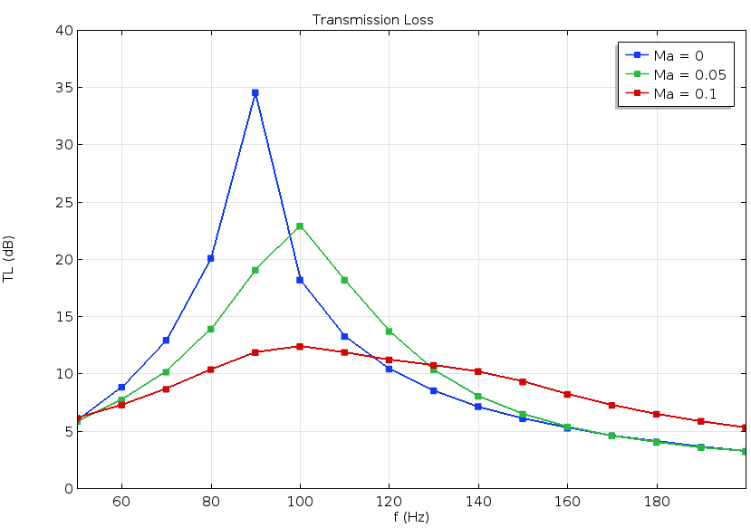
Transmission loss through the resonator as a function of frequency and Mach number of the background flow.
The pressure distribution inside the system at 100 Hz for Ma = 0.1. A plane wave is incident from the left side upstream of the flow.
Acoustic Liner with a Grazing Background Flow
In the Acoustic Liner with a Grazing Background Flow tutorial model, the acoustic liner consists of eight resonators with thin slits and the background grazing flow is at Mach number 0.3. The sound pressure level above the liner is calculated and shows good agreement with results from a published research paper (Ref. 2). This example computes the flow via the SST turbulence model in the CFD Module and the acoustic propagation with the Linearized Navier-Stokes, Frequency Domain interface. The acoustic boundary layer is resolved and the default linear discretization is switched to quadratic to improve the spatial resolution near walls.
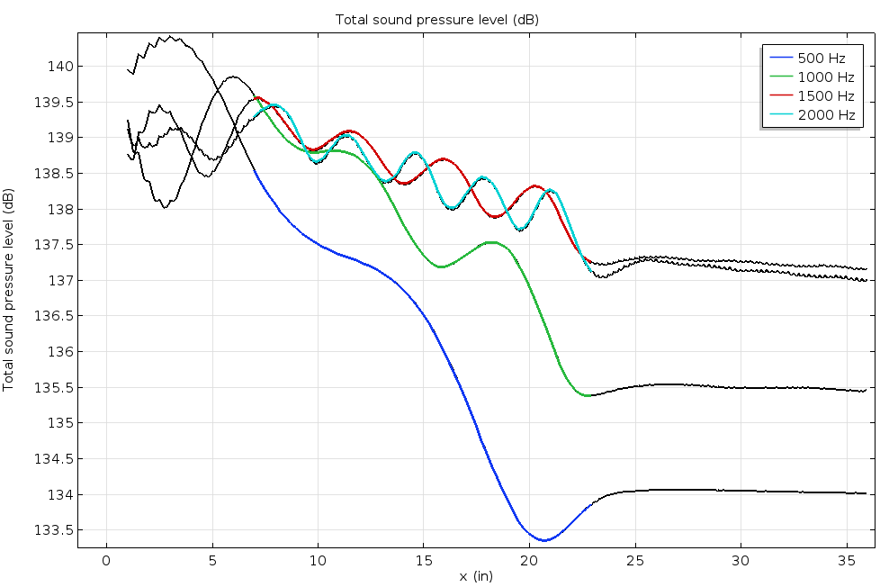
The curves show the sound pressure level on the surface above the liners for four driving frequencies. The colored part of the curves highlights the extent of the liner. These results show good agreement with the experimental results from the referenced research paper.
The acoustic velocity fluctuations as a plane wave propagates above the liners, showing the first four liners. The driving frequency is 1000 Hz. The color plot shows the velocity amplitude and the arrows show the velocity vector. Near the holes at the surface of the liner, vorticity is generated by the flow-acoustics interaction.
Coriolis Flow Meter
Coriolis flow meters — also called mass or inertial flow meters — can measure the mass flow rate of a fluid moving through it. This device can also compute the density of the fluid, hence the volumetric flow rate. The Coriolis Flow Meter tutorial model demonstrates how to model a generic Coriolis flow meter with a curved geometry.
As a fluid travels through an elastic structure (a curved duct, for instance), it interacts with the movement of the structure when vibrating. The Coriolis effect causes a phase difference between the deformation of two points on the duct, which can be used to determine the mass flow rate.
To model this, the Linearized Navier-Stokes, Frequency Domain interface is coupled to the Solid Mechanics interface via the built-in multiphysics coupling. As for the background mean flow, it is simulated with the Turbulent Flow, SST interface. Using this approach, FSI can be efficiently modeled in the frequency domain.
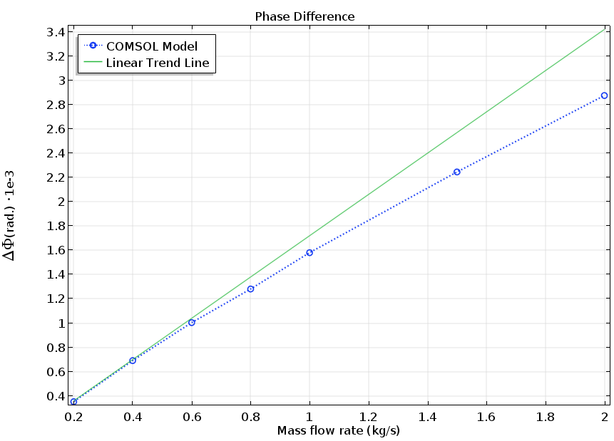
The phase difference between upstream and downstream points (red dots on the animation below). This curve represents the calibration results needed to run a Coriolis flow meter.
The movement of the Coriolis flow meter for three mass flow rates. The flow meter is actuated at the natural frequency of the structure, fd = 163.5 Hz. The deformation amplitude and phase are exaggerated for visualization. As the flow rate increases, the phase difference upstream and downstream increases.
Learn More About CFD and Acoustics Simulations in COMSOL Multiphysics®
- Check out these examples in the Application Gallery:
- Read this COMSOL Conference 2016 presentation: “Acoustic Scattering through a Circular Orifice in Low Mach Number Flow“
- Check out the COMSOL News 2017 — Special Edition Acoustics
References
-
E. Selamet, A. Selamet, A. Iqbal, and H. Kim, “Effect of Flow in Helmholtz Resonator Acoustics: A Three-Dimensional Computational Study vs. Experiments”, SAE International Journal, 2011.
-
C. K. W. Tam, N. N. Pastouchenko, M. G. Jones, and W. R. Watson, “Experimental validation of numerical simulations for an acoustic liner in grazing flow: Self-noise and added drag”, Journal of Sound and Vibration, p. 333, 2014.


Comments (16)
chen xu
August 15, 2017could you share how to use linearied navier-stokes interface in the aeroacoustic module to calculate noise of a jet engine or any example?please. i find this aspect example is very fewer.
Mads Jakob Herring Jensen
August 15, 2017 COMSOL EmployeeDear Chen Xu, as I stated in the beginning of the blog post the interface (the physics solved here) does not include flow induced noise, if this is what you are asking for. What you can do is to set up an analytical expression for a source and see how it propagates in the presence of a flow. See, for example, http://www.comsol.com/model/1844 or http://www.comsol.com/model/1371. Note that these models rely on another formulation of the governing equations. Best regards, Mads
Chen Xu
October 28, 2017hello, I have a question about CFD solution onto the acoustic domain. when boundaries have a symmetry edge, you add the constraint in the Helmholtz_resonator case. I don’t understand why V value is set to 0 in the first row in the Weak Form PDE. I spent much time to study the help but i can’t still resolve it. I hope you can help me. Thank you very much.
Patrick Flohr
March 6, 2018Hello,
Under Modeling Considerations it is stated:
◾Resolving the acoustic boundary layers: Consider if the modeled physical effects and the size of the model require that you resolve the acoustic boundary layers. If not, change from the default slip and isothermal conditions to no-slip and adiabatic options on walls.
My question: I understood that for resolving the boundary layers the NO-SLIP option is required. Is the statement above not suggesting the opposite?
Best regards,
Patrick
Mads Herring Jensen
March 6, 2018 COMSOL EmployeeHi Patrick
You are right, that is a typo. It should of course say “If not, change from the default no-slip and isothermal conditions to slip and adiabatic options on walls.”
I will make sure this is updated.
Thanks!
Best regards,
Mads
Phillip Springer
March 15, 2018Hi Mads,
could you share your source for Eq. (1), the linearized form of the hydrodynamic equations?
Cheers
Phil
Mads Herring Jensen
March 19, 2018 COMSOL EmployeeDear Phil
We have a detailed derivation of the equation in the theory section of the documentation for the acoustics module (and some references). It follows from a first order perturbation approach of the full NS equations. I believe that the form of the LNS equation we have implemented is very general with few assumptions – except for the linearity, of course.
Best regards
Mads
Robin Billard
April 8, 2020Hello Mads,
I’m currently using the LNS equations to investigate the behaviour of a Helmholtz resonator with a grazing flow. It is very similar to the example your showing except it’s in 2D.
I’m also using LiveLink to extract the matrices used to solve the LNSE in Matlab. I am using the stationnary solver.
From my understanding, COMSOL is solving the linear system AX = B in which
A = [K NF ; N 0]
X = [U ; lambda]
B = [L ; M]
with
K: the stiffness matrix,
NF: the constraint force Jacobian,
N: the constraint Jacobian,
U: the solution vector,
lambda: the Lagrange multipliers to impose the boundary conditions,
L: the load vector,
M: the constraint vector.
I managed to solve AX=B with Matlab and I obtained the same U as COMSOL.
I was hoping you could tell me how the LNSE are discretized, i.e. what is in K, NF, N, L and M.
I fathom L contains the sources and the edges integral resulting from the variational formulation and that K contains the domain integral from the variational forumlation.
Your help would be precious for my study.
Best regards,
R. Billard
成 严
October 27, 2021Dear Mads,
I got problems in using linear N-S equations to evaluate the Helmholtz Resonators when the neck is small, i.e. its diameter is 15mm. But, it woks when the neck is relatively big enough. What is the possible mistake I make?
Mads Herring Jensen
October 27, 2021 COMSOL EmployeeDear 成 严
There can be many causes to this. Please contact support, they will be able to help.
Best regards
Mads
Gustavo Silva
June 22, 2022HI, in this webpage: “https://www.comsol.com/model/coriolis-flowmeter-fsi-simulation-in-the-frequency-domain-51831” there is a model called :
“Coriolis Flowmeter: FSI Simulation in the Frequency Domain”
but notice there are two files:
1- coriolis_flow_meter_55.mph – 213.17MB
2- coriolis_flow_meter_55_cleared.mph – 0.44MB
why second file (2) of them is called ” cleared”, and is a lighter file than the first one file.
which are the differences.
And the second and most important question: IS THERE ANY STEP BY STEP FILE to do this simulation? there is just a general slide explaining the results of the model.
Thank you
Mads Herring Jensen
June 27, 2022 COMSOL EmployeeDear Gustave
The file “_celared” just means that the solution is cleared and you need to solve it again to look at the results. There are unfortunately no step-by-step instructions for this model. I invite you to open the model and look at the setup, boundary conditions etc. To get to know COMSOL we recommend that you try out some of the tutorial models in the application Library of COMSOL.
Best regards
Mads
Ekaterina Gudkova
February 8, 2023Hello! I have a question about Coriolis Flow Meter tutorial model. Is it possible to create a Coriolis flow meter model without using the acoustics module? And the second question: How to calculate model in the time domain?
Mads Herring Jensen
February 9, 2023 COMSOL EmployeeDear Ekaterina
You need the acoustics module to model the linearized N-S equations. You can switch the interface to the Linearized Navier-Stokes, Transient interface to model the response in the time domain.
Best regards
Mads
Ekaterina Gudkova
March 17, 2023Thanks for your reply. How to implement (or replace) PML in Linearized Navier-Stokes, Transient?
Sincerely, Ekaterina.
Mads Herring Jensen
March 17, 2023 COMSOL EmployeeThe only solution in the time domain is to use an impedance condition, probably with Z = rho*c, or something similar that includes a flow effect. Best regards, Mads