

In a previous blog post on optimizing battery performance, I focused on charging time and degradation in the context of the charging profile of a battery. In this blog post, I focus on maximizing the battery’s energy density during discharge by varying the positive electrode thickness and the active material volume fractions of both the positive and negative electrodes.
Editor’s note: Read the previous blog post, “Minimizing the Charging Time of a Battery”, to learn more about the relationship between charging time and battery longevity for a lithium-ion battery.
Modeling the Energy Density of a Lithium-Ion Battery
Let’s consider a lithium-ion battery model constructed using the Lithium-Ion Battery interface. The cell is simulated under a constant-current 1C discharge, and the model can be used to analyze the battery’s electrochemical behavior and performance. The cell consists of a graphite negative electrode and an NMC111 positive electrode, separated by an electrolyte-filled separator. The electrode thicknesses and active material volume fractions are specified as part of the porous electrode properties. For a given set of these parameters, the model predicts the cell voltage throughout the discharge and, consequently, the amount of energy the cell can deliver.
The energy delivered during discharge can be calculated by integrating the product of the cell voltage and applied current density over the discharge time:
The time integration can be implemented as an ordinary differential equation (ODE) in COMSOL Multiphysics version 6.4 and earlier, while in COMSOL Multiphysics version 2027, the functionality will be built into the Time Integral feature.
In this example, the cell current density, I, is set to correspond to a constant C rate, but, in principle, the maximization could be performed for any given discharge load profile.
Optimizing Electrode Dimensions
The electrode dimensions can be varied by changing the geometry and remeshing in every optimization iteration. However, by using the Deformed Geometry interface instead, the geometry can be modified by deforming the computational mesh, which allows the electrode dimensions to vary continuously without remeshing for each design configuration, helping maintain a smooth dependence of the model response on the geometric design variables. This condition makes the problem well suited for gradient-based optimization, which is particularly advantageous when working with many design variables.
In practice, the charges in the two electrodes should be balanced, and therefore the negative electrode thickness, L_\mathrm{neg} , is expressed in terms of the thickness of the positive electrode, L_\mathrm{pos} :
where:
- f_\mathrm{loss} = lithium inventory loss factor during formation
- \epsilon_{s,0}^\mathrm{neg}, \epsilon_{s,0}^\mathrm{pos} = negative and positive (initial) electrode volume fractions
- c_{s,\mathrm{max}}^\mathrm{neg}, c_{s,\mathrm{max}}^\mathrm{pos} = maximum negative and positive concentrations
- \mathrm{sol}_\mathrm{max}^\mathrm{neg} = maximum lithiation level in the negative electrode
- \mathrm{sol}_\mathrm{min}^\mathrm{pos} = minimum lithiation level in the positive electrode
To gain a deeper understanding of how to balance electrodes and see other example models, view this blog post.
The battery design variables are limited to the thickness of the positive electrode, L_\mathrm{pos}, and the initial volume fractions of the negative and positive electrodes, \epsilon_{s,0}^\mathrm{neg} and \epsilon_{s,0}^\mathrm{pos}.
Solver and Optimization Settings
The partial differential equations (PDEs) for the electrolyte potential, electrolyte salt concentration, and the electric potential are solved with a time-dependent solver. Here, the backwards differentiation formula (BDF) is used, then terminated when the insertion particle concentration at the boundary between the negative electrode and the separator falls below the minimum lithiation level. The method of moving asymptotes (MMA) is used as the optimization solver. Robustness is improved using the Move limits option, which limits the change of design variables between optimization iterations.
Results
The objective history is plotted with and without shape optimization in the figure below. The shape optimization improves the objective from 2.5 to 3.2 J/m3, although this improvement depends on the initial values of the design variables.
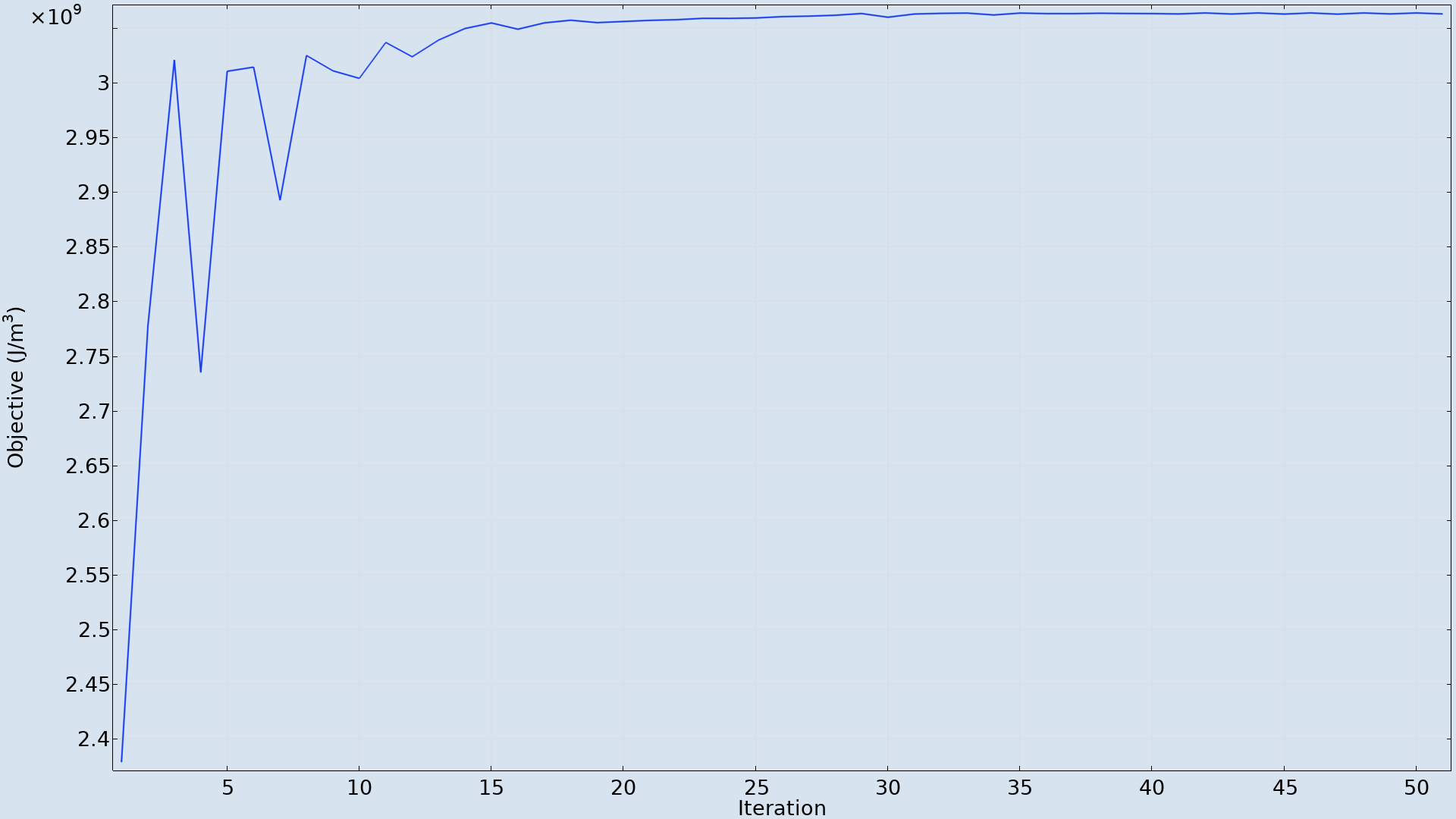 The objective history shows that 50 iterations of the MMA solver are sufficient.
The thickness of the positive electrode and the positive and negative electrode volume fractions are plotted below. Compared to the initial values, the optimized battery has significantly denser electrodes (that is, with larger electrode volume fractions). In this way, the energy density gets larger since the electrodes can store more lithium per volume. The electrode volume fractions may however not become too high, since this at the same time reduces the electrolyte volume fraction of the porous electrodes. This in turn reduces the effective ion transport capabilities of the electrolyte.
Similarly, slightly thicker electrodes can contribute to a higher energy density in the optimized battery by increasing the amount of active material. However, the electrodes should not be made too thick, since increasing the electrode thickness also increases the ion transport distance through the electrolyte phase. The resulting transport limitations can lead to larger concentration gradients and increased polarization, reducing the usable capacity and energy of the cell.
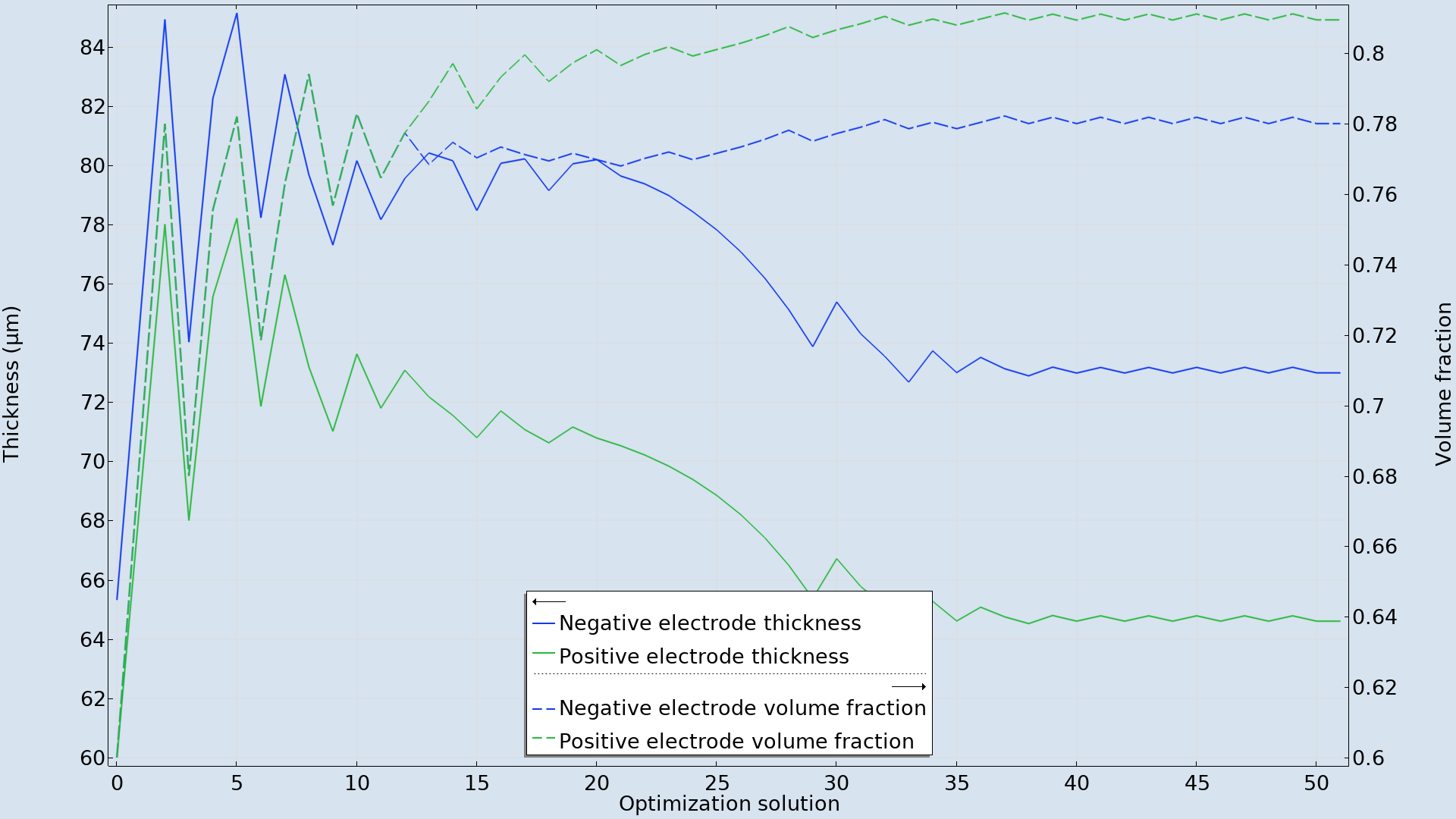 The optimization results in higher active material volume fractions and slightly thicker electrodes.
Takeaways
In this example, optimization is used to improve the battery energy density by varying the active material volume fractions and the thickness of the electrodes.
More generally, COMSOL Multiphysics facilitates gradient-based optimization of fully coupled multiphysics problems. Different optimization approaches can also be combined within the same model, including parameter, shape, and topology optimization as well as optimal control.
Next Steps
- Interested in the details of this model’s setup in COMSOL Multiphysics?
- Download and explore it for yourself: Maximizing the Energy in a Lithium-Ion Battery
- Want to learn more about optimization?
- View this tutorial model from the COMSOL Application Gallery about minimizing a lithium-ion battery’s charging time.
- Check out these previous blog posts.



Comments (0)