
Guest blogger Björn Fallqvist from Lightness by Design continues a two-part discussion on estimating hyperelastic material parameters with a lap joint shear test, and subsequently implementing a damage model to replicate softening behavior. You can read Part 1 here.
Mathematical Background of the Damage Model
To model the damage for a hyperelastic material, we modify the strain energy density function by a damage variable \omega; i.e., the strain energy density is now defined as \omega \psi. By definition, \omega = 1 in the undamaged state and \omega = 0 when the material is fully ruptured. It can be noted that this is different from the customary definition of unity minus the damage variable, but equivalent. The evolution law can just as well be written in such a form, albeit with a sign change.
We make use of a previously defined evolution law (Ref. 1) to model the evolution of damage on rate form according to:
where \beta and b are material parameters.
The physical basis for this equation is derived from Arrhenius’ law, which states that the rate of a reaction (in this case, breaking of chemical cross-links) is an exponential according to:
Here, k is the reaction rate constant, A is a pre-exponential factor for each chemical reaction, R the universal gas constant, T absolute temperature, and E_b the reaction activation energy (depth of the cross-link potential well).
If we were to consider the additional energy due to imposed deformation, this can be rewritten:
The reaction k is the rate of cross-link bonds breaking, and we assume that the rate of damage is proportional to this. Also, we conjecture that the damage rate must be proportional to how many bonds can be broken at a certain time; i.e., the current state of the material \omega. We then end up with the evolution law defined first in this section. The parameter b can be seen as a fraction of strain energy (per concentration unit) available to break bonds. The idea is illustrated in Figure 1 (Ref. 2).
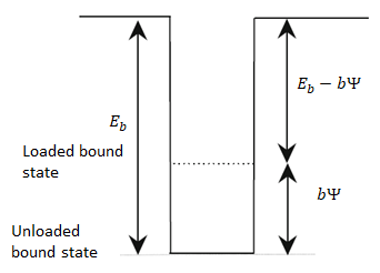
Figure 1. Bound state for cross-linked molecules. To escape the potential well in the loaded state, the energy required to break the bond is E_b-b\psi. Image from Ref. 2.
The internal dissipation D_{int} must be greater than or equal to zero to be thermodynamically valid, according to:
Thus, the evolution law is valid, with the restriction that \beta \geq 0.
Implementing the Damage Model in COMSOL Multiphysics®
Since the damage evolution law is a first-order differential equation, it is easily defined in the COMSOL Multiphysics® software by inserting an ODE object, shown in Figure 2, for the adhesive domain. The initial value of \omega is set to unity (no damage). The reference temperature parameter is set to 20°C (293 K).
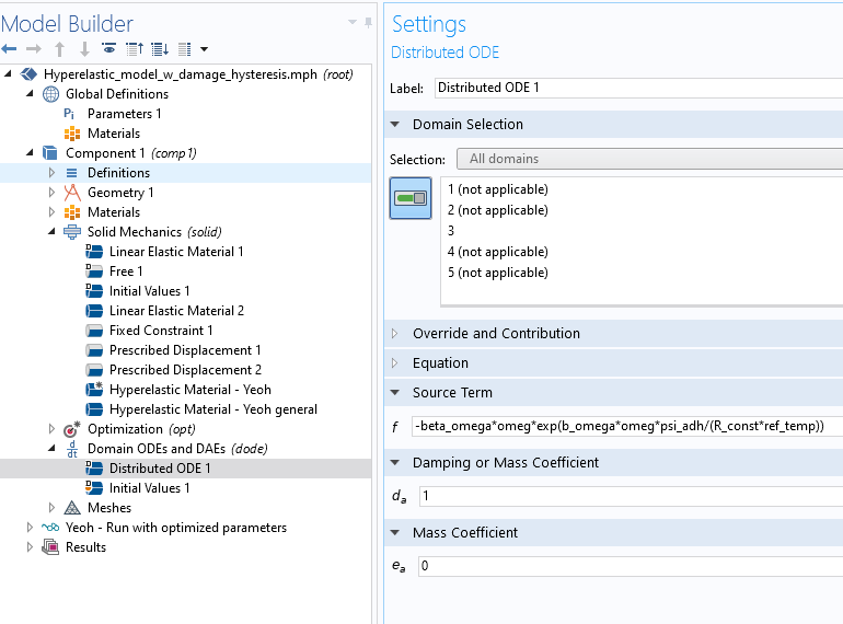

Figure 2. Domain ODE definition for damage evolution.
The damage variable “omeg” is used in the hyperelastic material definition, as described in the previous blog post, and \psi_{adh} is defined as a solution variable, as shown in Figure 3.
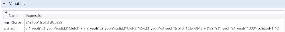
Figure 3. Definition of strain energy density function used in ODE definition.
The optimization is set up as described previously, although more points are now selected for optimization in the least-squares objective. The two new damage model parameters are added as control variables; see Figure 4.

Figure 4. Setting up optimization, including damage evolution.
In an initial analysis, we choose to use the points at 2, 6, 10, and 13.5 mm. Then, in a second analysis, we use all points, using the optimized values from the initial analysis as starting points. The parameter values (and results) presented are taken from this second analysis with all data points.
Results: Optimized Material Parameters for the Hyperelastic Model with Damage
Optimized Parameters and Force-Displacement Curve
The initial and optimized material parameters for the model with damage can be seen in Table 1.
| Scaling Parameter | Initial Value [-] | Optimized Value [-] | Damage Parameter | Initial Value | Optimized Value |
|---|---|---|---|---|---|
| s_{f1yeoh} | 9.980 | 10.62 | \beta | 3.27e-2 [1/s] | 4.24e-2 [1/s] |
| s_{f2yeoh} | 0.366 | 0.403 | b | 4.81e-4 [m3/mol] | 4.12e-4 [m3/mol] = 0.41/M |
| s_{f3yeoh} | 0.260 | 0.203 | |||
| Least-squares objective [N2] | |||||
| 121570 |
The force-displacement curve for this analysis is shown in Figure 5.
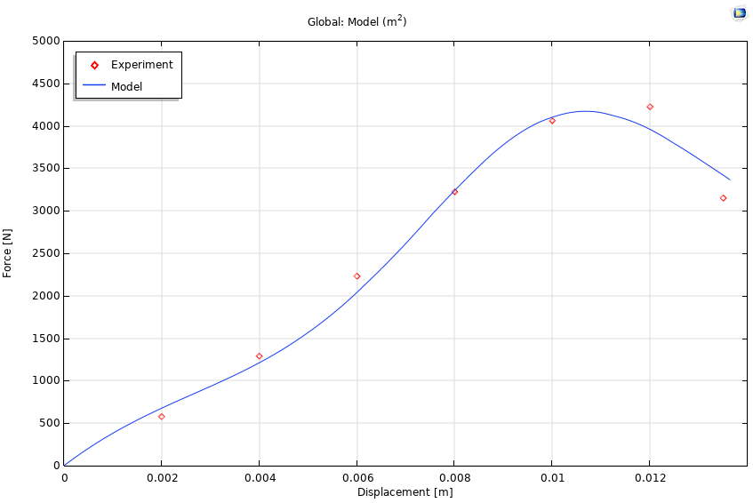
Figure 5. Force-displacement curve for hyperelastic model with damage.
There is significant softening at larger strains, and the damage evolution captures a softening of the material, although there is some discrepancy between experimental data and model predictions. The parameter b is a fraction per cross-link concentration, and for each molar concentration M, approximately 41% of the total strain energy is used for breaking cross-link bonds.
Strain-Rate Dependence
Due to its rate form, the evolution law captures strain-rate effects. For comparison, the previous analysis is run with an end displacement rate of 130 mm/min, cf, as shown in Figure 6.
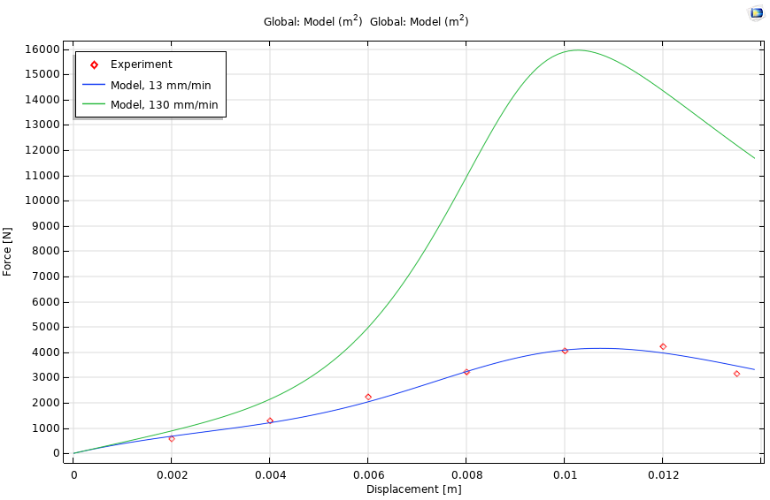
Figure 6. Effect of deformation rate.
A higher deformation rate implies that damage is given less time and opportunity to evolve. This is also true for Arrhenius’ law, which gives the probability per time unit that a chemical reaction will occur, in this case cross-link debonding.
Hysteresis and Material Cycling
In the following section, the material parameters defined in Table 1 are used for analysis.
A common phenomenon observed in soft materials is hysteresis; i.e. the loading and unloading paths do not coincide due to energy dissipation in the material. This manifests itself as a stress-strain curve that changes over each cycle and often stabilizes after a certain degree of softening (or hardening). The damage model presented herein captures hysteresis, evident if we also include unloading in the analysis; see Figure 7.
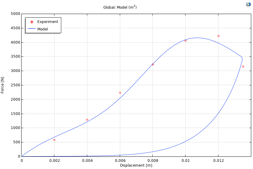
Figure 7. Hysteresis curve. Unloading occurs at the same rate as loading.
To further illustrate, we assign a prescribed 7.5 mm end displacement as a sine wave, with a frequency 0.25/s (i.e., a full cycle in 4 s). The force-displacement curves for the five initial cycles are shown in Figure 8.
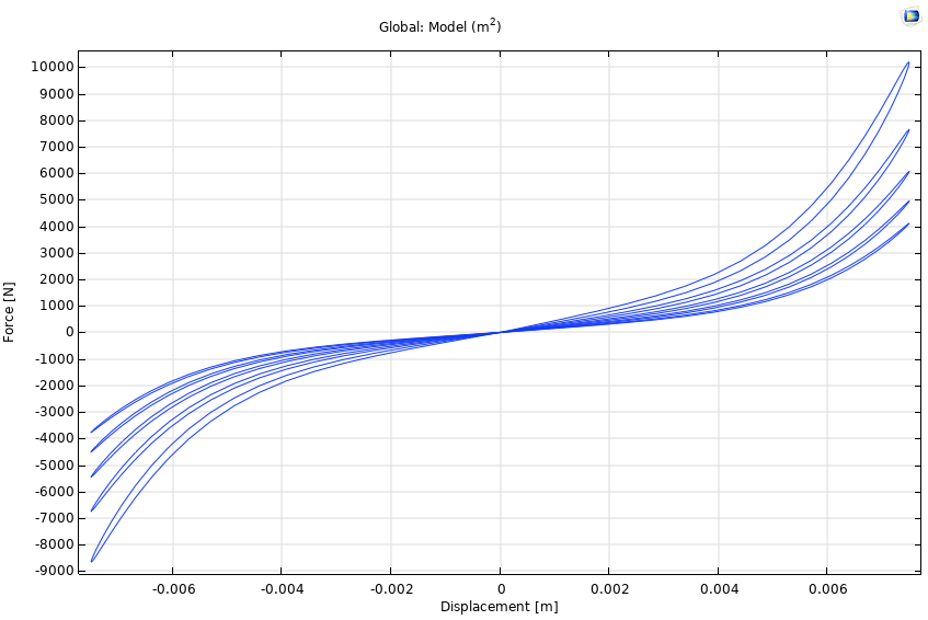
Figure 8. Hysteresis curves for five initial cycles.
Significant softening can be observed, and the loading-unloading paths do not coincide. Due to the original form of the damage evolution law, there is no stabilization of the curves. This can also be seen if we decide to assign a sinusoidal force of 6000 N with the same frequency. In Figure 9, the displacement at the plate end keeps growing.
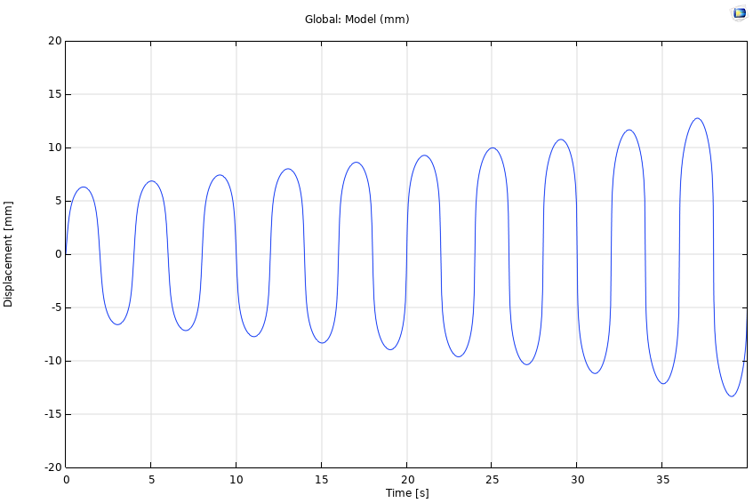
Figure 9. Displacement for a sinusoidal force of constant amplitude.
The displacement of the material is shown at times 1, 13, 25, and 37 s in Figure 10.
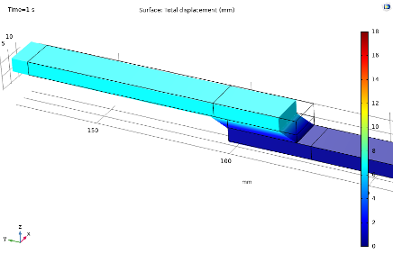
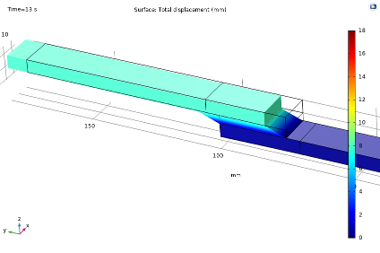
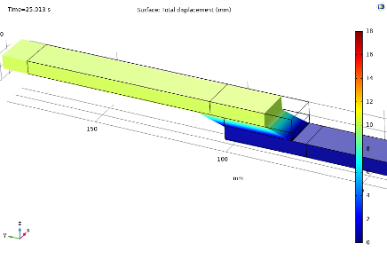
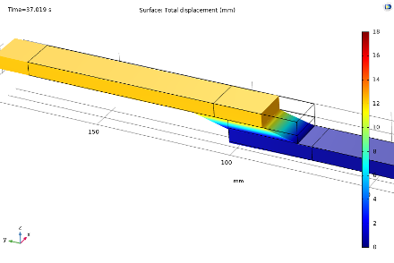
Figure 10. Displacement at times 1, 13, 25, and 37 s during cycling.
If we wish to implement stabilization of the material curves after cycling, we may do so by modifying the damage rate equation with an exponential decaying function:
\begin{cases}
\-\beta \omega e^{(\frac{b \omega \psi}{RT})},\qquad \qquad \qquad \qquad \quad \omega > \omega_t\\ -\beta \omega e^{(\frac{b \omega \psi}{RT})}e^{({-\omega_{t,rate}|\omega-\omega_t|})}, \quad \omega \leq \omega_t
\end{cases}
where \omega_t is a threshold value for the material damage state below which damage should not occur.
The factor \omega_{t,rate} governs how quickly the damage rate decays below the threshold value. This form is needed, since simply setting the rate to zero below the threshold value results in discontinuity convergence problems. Using the same analysis as for Figure 8, but with \omega_t=0.6, and \omega_{t,rate}=1000, the cycle hysteresis curves are as shown in Figure 11.
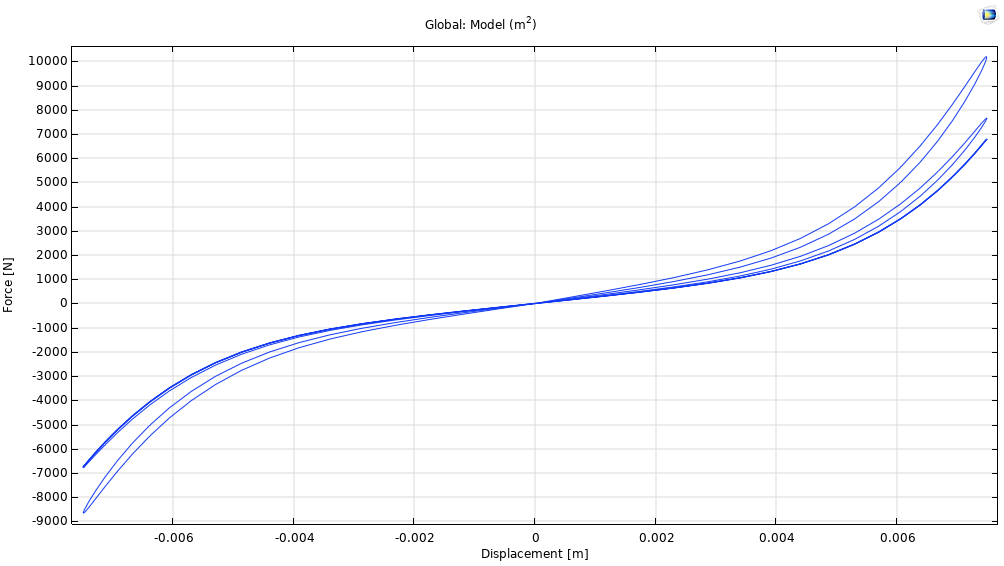
Figure 11. Hysteresis curves for five initial cycles, with \omega_t=0.6, and \omega_{t,rate}=1000.
A clear stabilization of the material response can now be seen during the second cycle.
The proposed damage evolution law has three parameters (\omega_{t,rate} can merely be set to 1000), and incorporates the following effects:
- Hysteresis
- Material softening/rupture during monotonic loading
- Cyclic material softening
- Strain-rate dependence
- Creep
Conclusions and Final Thoughts
We have demonstrated how material parameters can be determined from a lap joint shear test, using a combination of the Solid Mechanics and Optimization interfaces in COMSOL Multiphysics. Any rate-based damage law could easily be implemented in a similar way by operating directly on the user-defined strain energy function.
We have also seen that the number of points, and which points we use, for our optimization will affect the results. Given the same initial values, optimizing for all data points results in a poor curve fit. As explained prior, the final values from an optimization with every second point were instead used as initial values in a second analysis. The data point with the highest recorded force was also included in the second analysis to slightly improve the fit. It is easier to optimize with respect to evenly spaced points, so if a least-squares fit of a curve is problematic, one may try to choose fewer points that are roughly evenly spaced in order to obtain good initial parameter values.
The damage evolution law implemented herein is appealing thanks to its ease of implementation. It establishes a dependence between applied deformation (strain) rate and stress, along with cyclic and monotonic softening, as well as creep effects.
The stabilization of the material response curves has been shown to be possible to replicate by including a threshold value for the damage evolution. This could be thought of as a percolation threshold and that the network has been disrupted to such an extent that there is not sufficient connectivity between polymer chains to fully transfer mechanical loads between cross-links and break them. Other modes of deformation then govern the macroscopic behavior, such as filament entanglement and entropic stiffness. The inclusion of a threshold value is mainly of interest in applications where the material is to be cycled. For monotonic loading, where the material will rupture at large enough deformation (such as the test modeled in this blog series), the distinction between the two types of mechanisms is blurred, and the damage law can be used in a phenomenological sense.
An alternative threshold definition could be the strain energy density, although this does not easily lend itself to a physical representation of the microstructure, and selecting a threshold value is not straightforward.
For certain classes of materials, such as biological tissues, it is also desirable to implement reversible viscoelastic behavior. This could be done, for example, by replacing the isochoric first invariant in the hyperelastic formulation with its elastic counterpart, and assigning evolution laws for the viscous deformation, cf. (Ref. 2). One then ends up with a material formulation with different time scales for reversible and irreversible deformation.
Thermal effects can be included in the damage model, thanks to the temperature variable in the expression for the evolution rate. But this would primarily be of interest in creep applications at a constant temperature, since the material parameters can also be expected to be dependent on this.
About the Author
Björn Fallqvist is a consultant at Lightness by Design working with product development based on numerical analysis. He obtained a PhD from the Royal Institute of Technology in 2016, working with developing constitutive models to capture the mechanical behavior of biological cells. His main professional interest and specialization is in the fields of material characterization and using various material models to capture physical phenomena.
References
- B. Fallqvist, M. Kroon, “Constitutive modelling of composite biopolymer networks”, Stockholm: Journal of Theoretical Biology, vol. 395, 2016.
- B. Fallqvist, M. Kroon, “A chemo-mechanical constitutive model for cross-linked actin networks and a theoretical assessment of their viscoelastic behaviour”, 2, Stockholm: Biomechanics and Modeling in Mechanobiology, vol. 12, 2013.


Comments (2)
Valery Anpilov
September 8, 2020Very useful information !
Buccma Accumulator
July 14, 2023Thank you for your wonderful article it helps me a lot.