
From time to time, we encounter periodic structures in RF applications, such as frequency selective surfaces (FSS), electromagnetic band gap (EBG) structures, reactive impedance surfaces (RIS), high impedance surfaces (HIS), and metamaterials. If you address an entire periodic problem in a simulation, it involves a high computational cost and long computation time. In this blog post, we will show how to simplify complicated numerical models using periodic boundary conditions with several examples from the RF Module Application Library.
Using Periodic Conditions to Simplify Your RF Models
In the Mirror Room at the World Expo in Milan, Italy, the mirrors generate countless building images. This is a good example of the periodic condition.

Michelle Obama in the Mirror Room at the World Expo. Image in the public domain, via Wikimedia Commons.
The simulation process of periodic structures can be streamlined by choosing proper numerical representations and minimizing the computational model size. When there is a structural pattern repeatedly observed in an electromagnetic model, the entire model can be scaled down to a single basic cell with periodic conditions. Applying the periodic condition on a pair of boundaries in the single-cell model creates a virtually infinite array along the axis connecting the pair of boundaries.
The microwave absorbers used in an anechoic chamber can also be analyzed without including the entire room.
To characterize the absorbers used in the anechoic chamber, only a single cell is needed with the Periodic boundary condition on all side walls.
When modeling electromagnetic waves and periodic structures, diffractions and higher-order modes can be critical for periodic cells in which the unit single cell size is comparable to the wavelength. However, for subwavelength periodic structures, model complexity is only marginal.
Periodic Boundary Condition Examples
In the RF Module Application Library, you can see a few examples that demonstrate how to utilize the Periodic boundary conditions with a single unit cell to perform more efficient simulations.
Reflection and Transmission Coefficients Between Two Media
The Fresnel equation model describes wave propagation in two media infinitely extended on the xy-plane. Modeling a small portion with Periodic boundary conditions does not sacrifice the accuracy of the computation. With a port excitation, reflectivity and transmittivity are calculated from the S-parameters.
Left: The y-component of the electric field plot, with averaged power flow arrows when the angle of incidence is 30 degrees. Right: The Periodic condition is applied to a pair of boundaries. The other pair of side walls is configured to be a perfect electric conductor.
Frequency Selective Surfaces (FSS)
The frequency responses of periodic structures such as FSS, RIS, HIS, and EBG metamaterials can also be studied using Periodic boundary conditions. Port features combined with perfectly matched layers (PML) compute the S-parameters without distortion from any possible higher-order modes caused by the periodic structures.
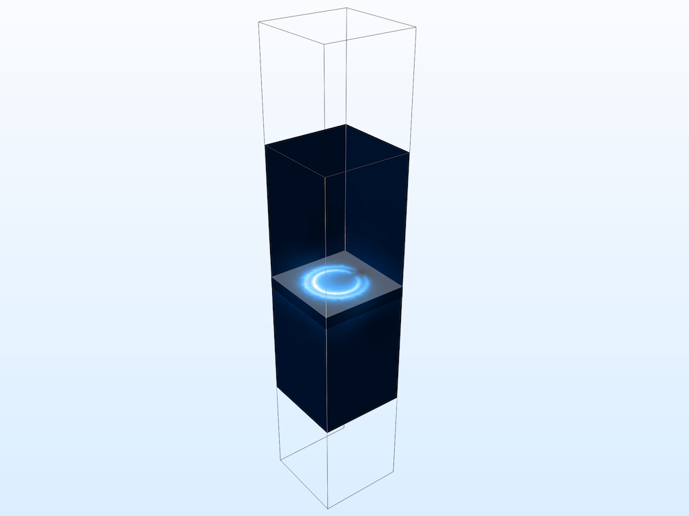
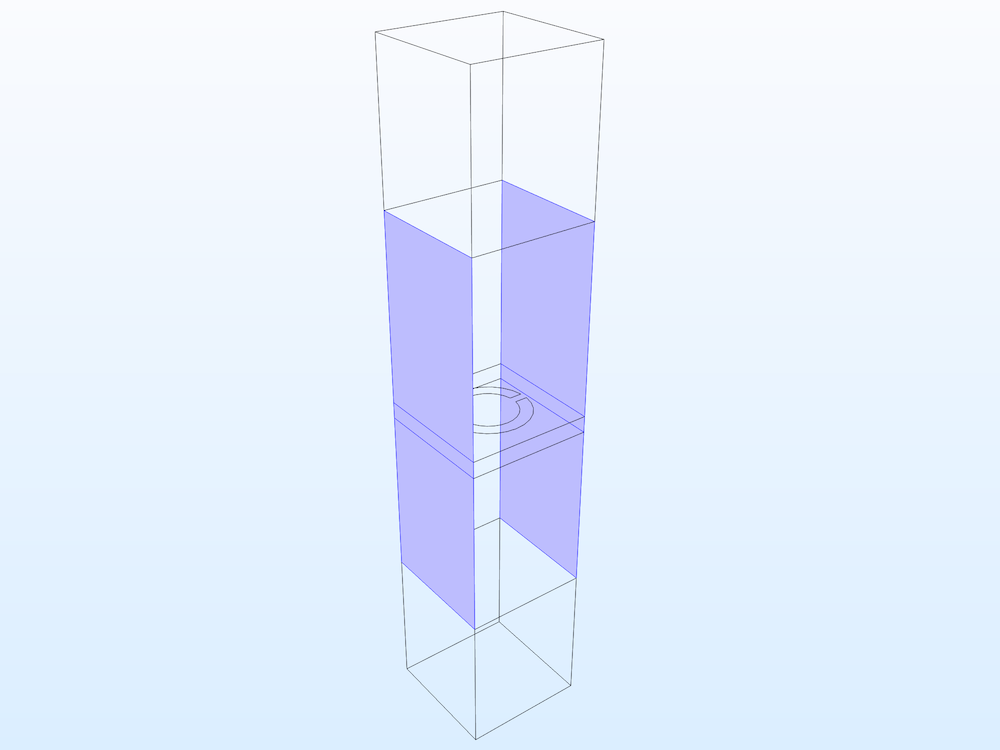
Left: The electric field norm is plotted at the resonant frequency. Right: The model requires a total of four sets of Periodic boundary conditions.
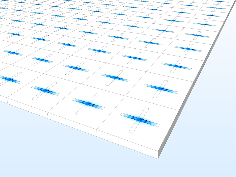
The Frequency Selective Surface Simulator application offers several types of predefined unit cell configurations, such as circle, ring, split ring, rectangle, and cross.
Microwave Absorbers
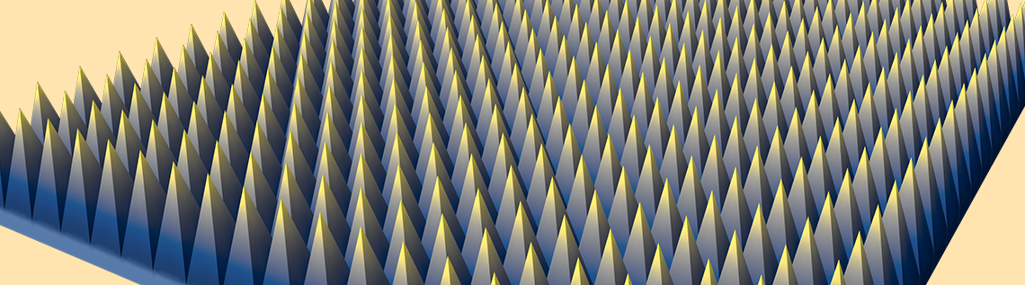
When characterizing radiating devices, tests and measurements are performed in a conventional anechoic chamber. The walls, floor, and ceiling of the room are finished with microwave absorbers that absorb and attenuate incident fields to minimize the reflections. This creates a virtually infinite space, and the device under test (DUT) can be evaluated without external signal distortions.
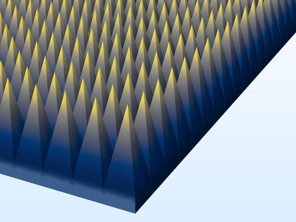
How would you address the numerical modeling of an infinite array of pyramidal absorbers without Periodic boundary conditions?
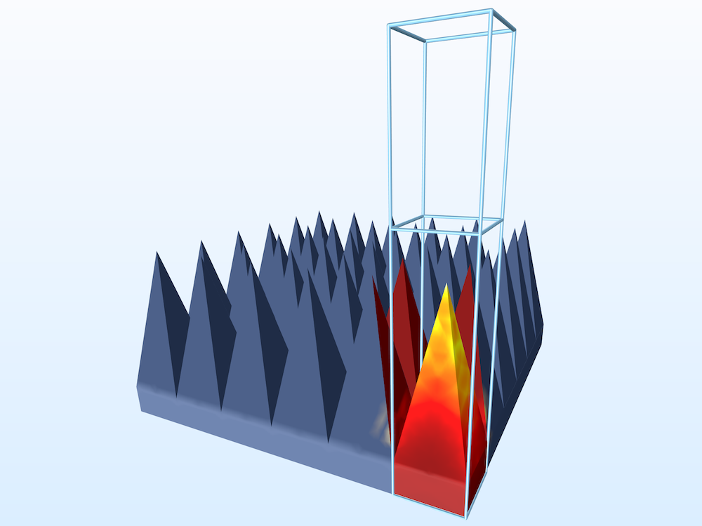
The entire wall of the chamber does not have to be part of the simulation to analyze and enhance the performance of the absorber. A single pyramidal cell with a Port boundary condition, as well as Periodic conditions, computes the reflectivity and field attenuation inside the pyramidal structure.
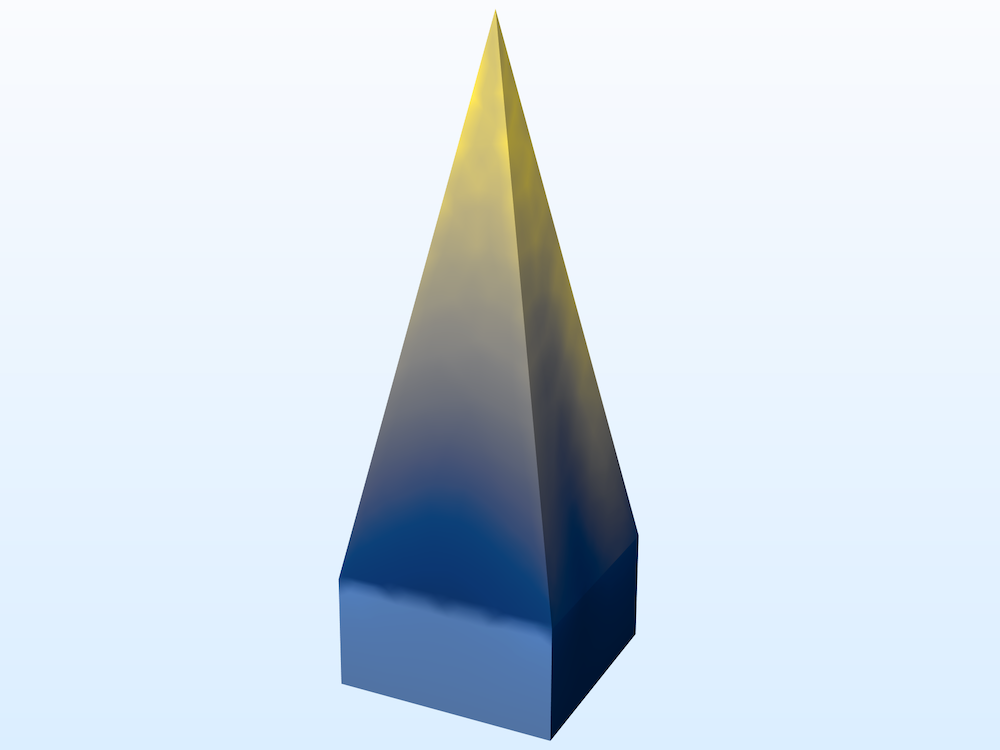
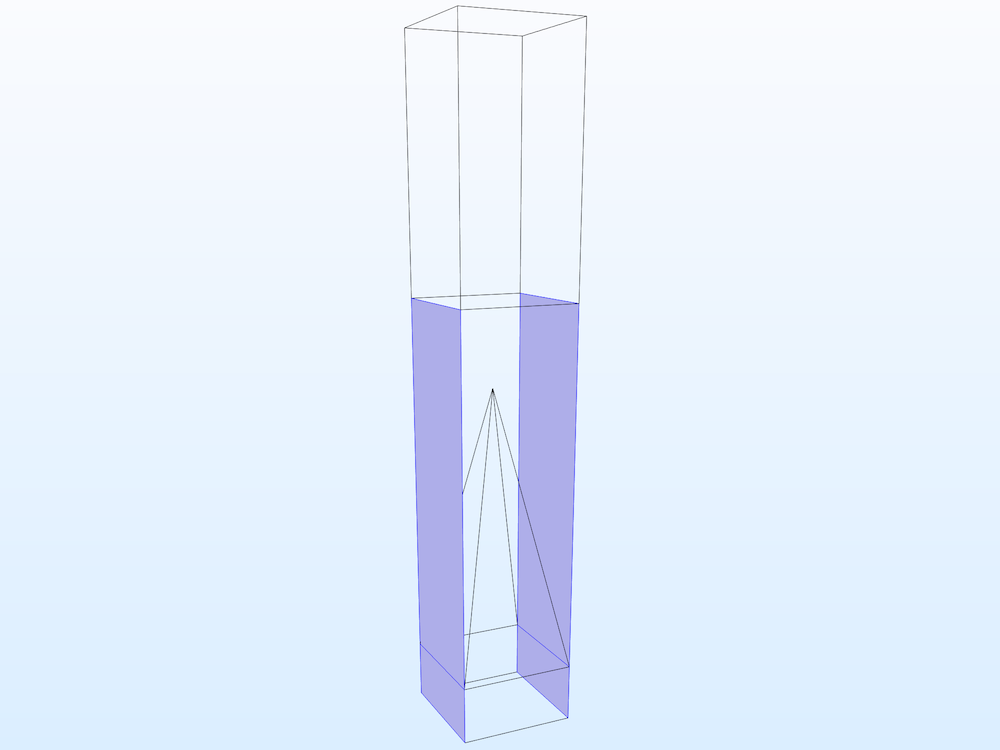
Left: The electric field norm on the surface of the pyramidal absorber when there is a 30-degree incidence wave. Right: The model requires a total of four sets of Periodic boundary conditions.
Plasmonic Wire Grating
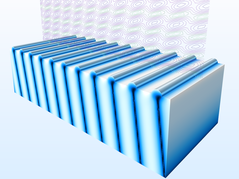
If physical phenomena can be represented by Maxwell’s equations, the numerical analysis in the RF Module is not limited to RF, microwave, and millimeter-wave applications and can be extended to terahertz and lightwave areas. In this surface plasmon-based circuit plasmonic wire grating model, the coefficients of refraction, specular reflection, and first-order diffraction are computed as functions of the angle of incidence for the grating on a dielectric substrate using Periodic conditions and Port features.
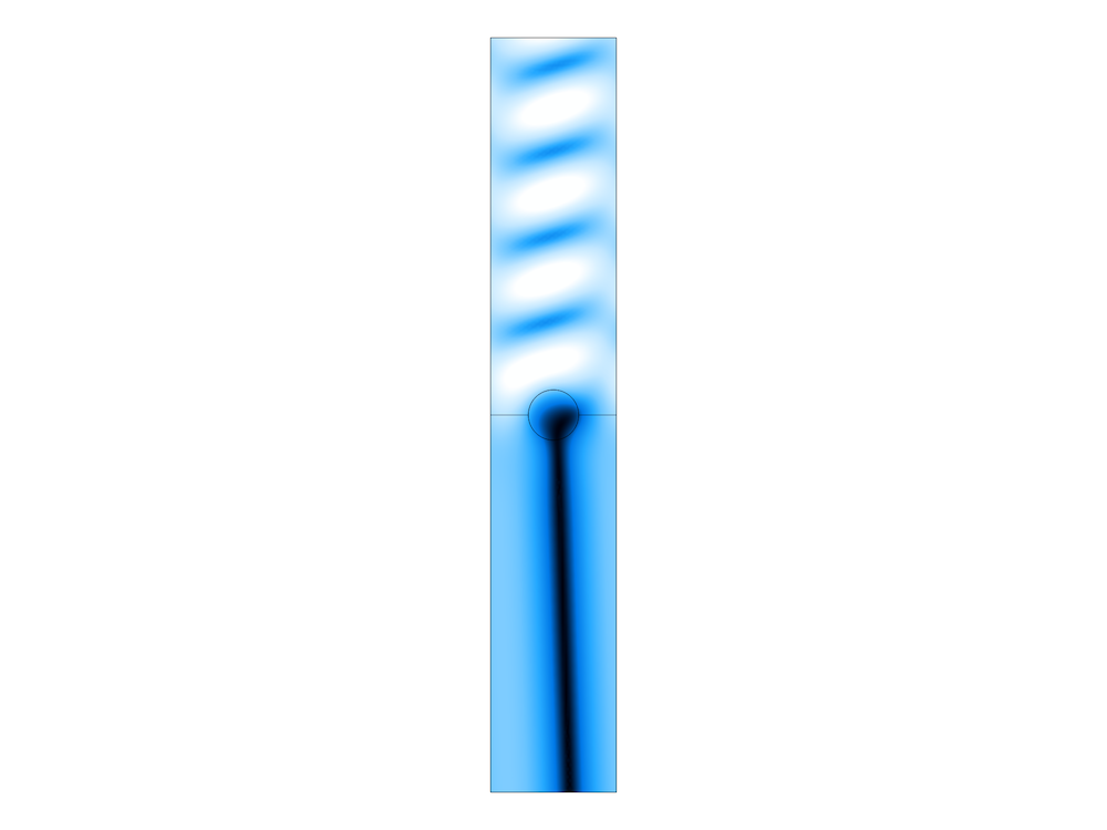
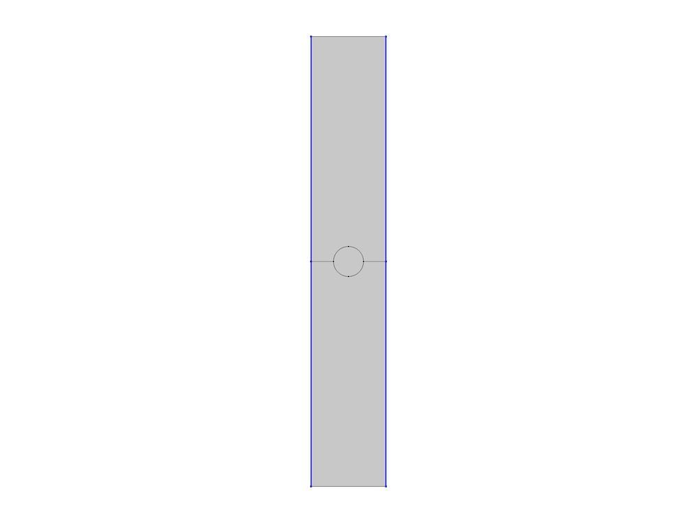
Left: The electric field norm plot at a 36-degree angle of incidence. Right: The Periodic boundary condition generates an infinite array of the wire grating.
Some Notes on Using Periodic Conditions
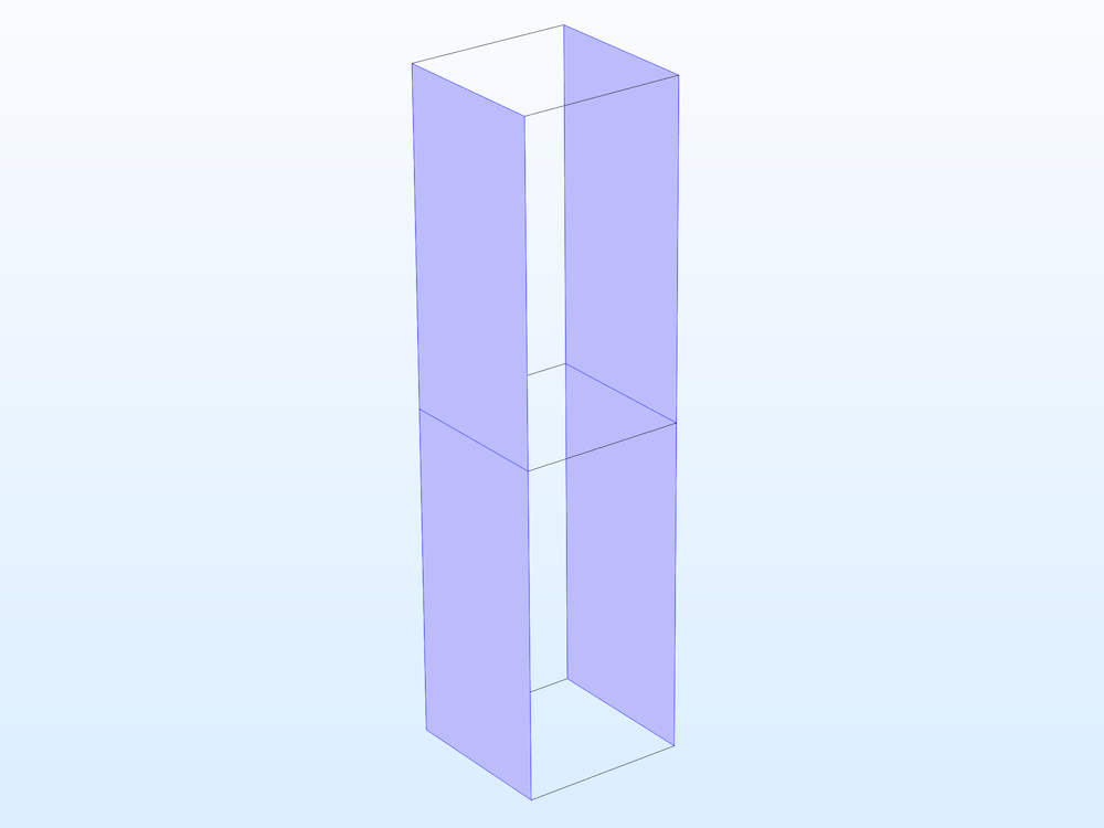
The boundary selection of a Periodic condition consists of a pair of boundary sets with an identical geometry shape, where we connect two surfaces with the following numerical conditions:
- Continuity (\mathbf{E}_{\mathrm{destination}} = \mathbf{E}_{\mathrm{source}})
- Anticontinuity (\mathbf{E}_{\mathrm{destination}} = -\mathbf{E}_{\mathrm{source}})
- Floquet (\mathbf{E}_{\mathrm{destination}} = \mathbf{E}_{\mathrm{source}} e^{-j \mathbf{k}_{\mathrm{F}} \cdot (\mathbf{r}_{\mathrm{destination}}-\mathbf{r}_{\mathrm{source}})})
The magnetic field relation between the source and destination boundary selections is the same as that of the electric field.
With the Continuity option, two surfaces have the same solution, while the Anticontinuity option provides out-of-phase solutions between two selections. The Floquet option is the most versatile, as it allows us to have an arbitrary phase variation between two sets of boundaries, so we can handle the computation with a various angle of incidence.
When the mesh of a model with Periodic boundary conditions is generated through the physics-controlled option, each set of the pair associated with the Periodic condition is set to have a mesh that is identical to the other set of the pair behind the scenes. Identical mesh from one surface to the other surface can be created using the Copy mesh option. By changing the option from Physics controlled to User defined in the Mesh node, the mesh sequences used for the physics-controlled mesh are populated on the Mesh node. You can see that Copy mesh is applied to the Periodic condition boundaries.
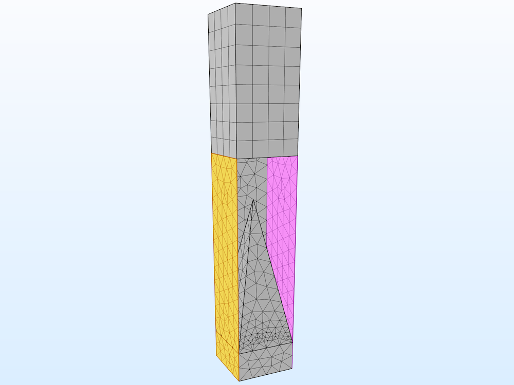
Using the Copy mesh feature, an identical mesh can be created between the source and destination boundary selections.
One of the advantages of using COMSOL Multiphysics is that you can have full control over the mesh generation in your periodic RF models. If you build a mesh from scratch, you have to make sure that the identical mesh is built on the pair of boundaries in the Periodic condition’s boundary selection.
Creating Appealing Visualizations of Periodic RF Models
You might already notice that some of the examples in the RF Module Application Gallery, as well as those mentioned above, have quite attractive results plots that are different from the original single-cell geometry. The Array 3D dataset helps you plot the finite array figures without duplicating the single cell illustration repeatedly. Go to Results > Data Sets and right-click to get to the Context menu. The dataset is available by selecting More 3D Data Sets > Array 3D.
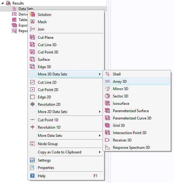
The Array 3D dataset is available from the Context menu under the Data Sets node.
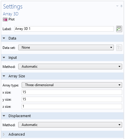
Choose the number of arrays you prefer for your presentation.
After adding Array 3D in the Data Sets node in the Model Builder, you can set the number of the array you want to plot using the results of the single cell in the Advanced section. When visualizing solutions in a 3D plot, make sure that you set the current dataset to Array 3D.
When zooming into the simulation model to have a closer look, try using the CTRL key while clicking the mouse wheel. This method changes the camera view settings and gives the look and feel of a 3D perspective.
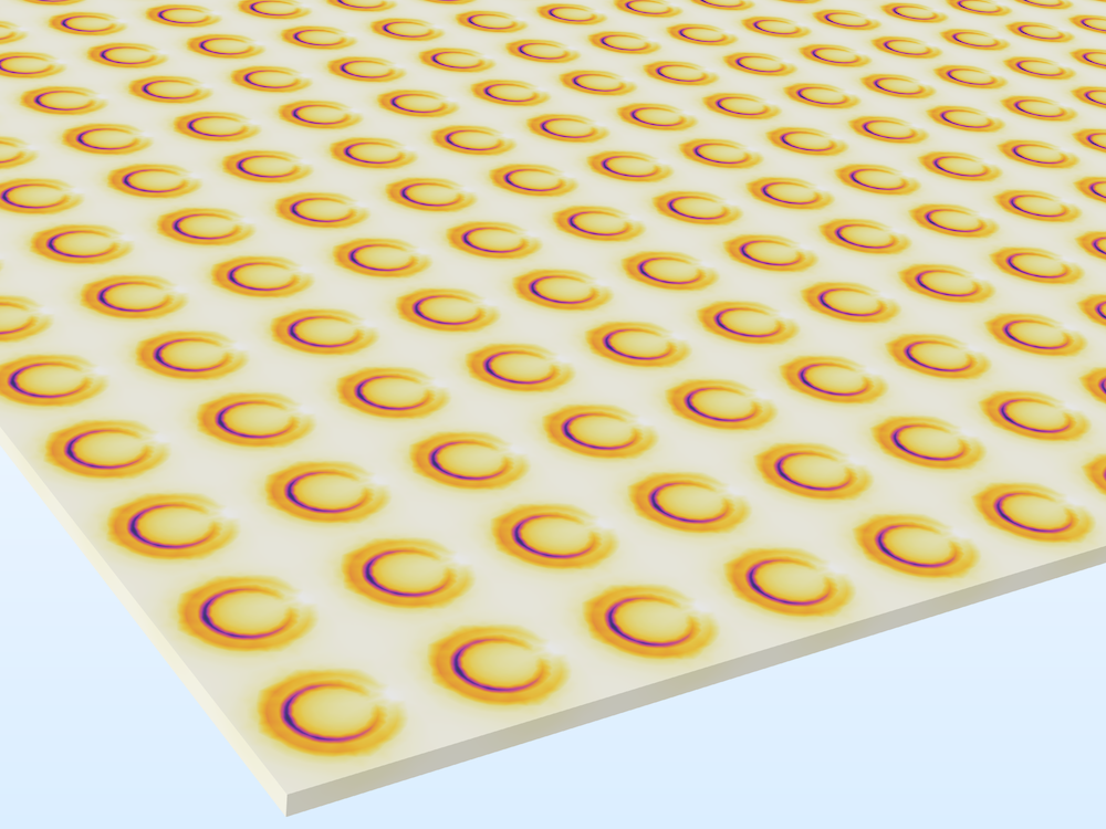
A frequency selective surface. The Filter subfeature of a volume plot allows you to plot the user expression on a chosen area. The Plot dataset edge in the Plot settings section of the 3D Plot Group is unchecked.
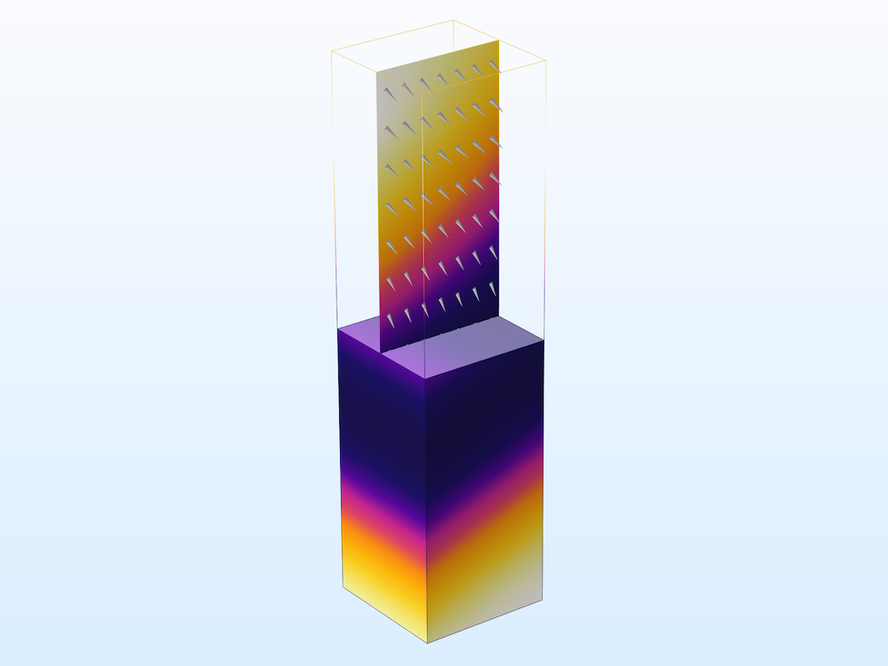
The field norm plot in the Plasmonic Wire Grating Analyzer simulation application. The 3D visualization is generated from the 2D model simulation results.
If you are interested in plotting a phase-varying field rather than the norm of the field, go back to the array dataset settings, activate Floquet-Bloch periodicity in the Advanced section, and type the Wave vector value. For the Plasmonic Wire Grating model in the RF Module, use the expression emw.kPeriodicx in the Array 2D dataset.
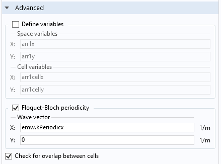
In the Advanced section, Floquet-Bloch periodicity activates the incremental user-specified phase variation.
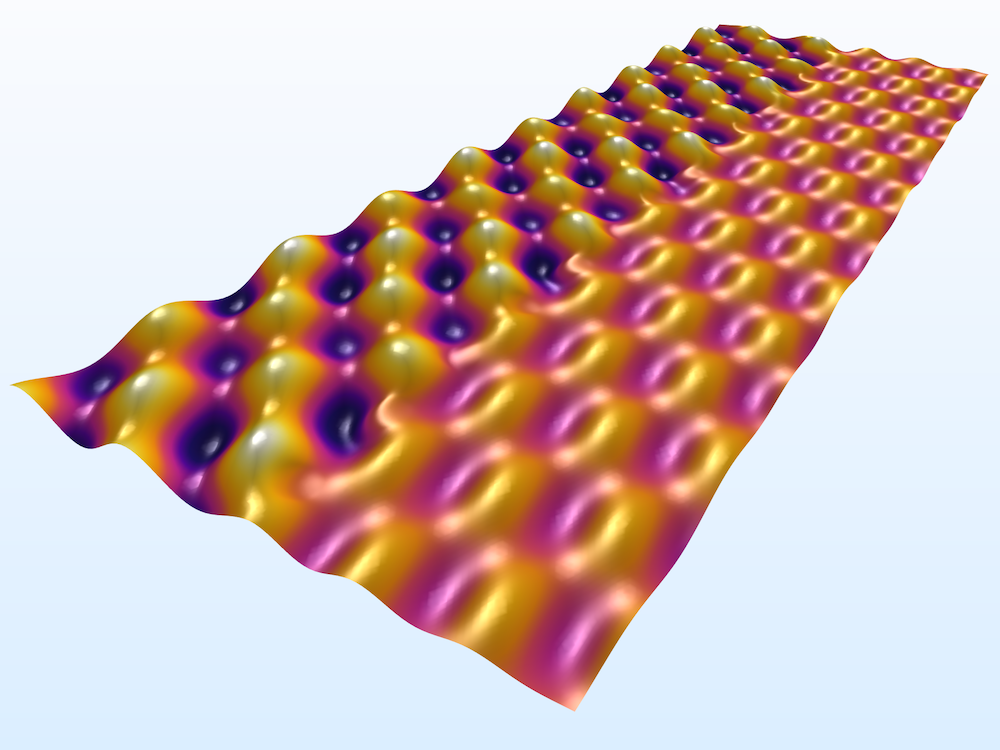
The z-component of the electric field in the Plasmonic Wire Grating model with phase progression in each array cell. A 15-by-1 Array 2D dataset is used and Height Expression is added on the surface plot.
Concluding Remarks
The Periodic boundary condition is the key to modeling various infinitely periodic structures in RF applications. Since it is not necessary to include the entire periodic structure in the simulation domain with this boundary condition, only a single unit cell, computing the subwavelengths won’t require a lot of computational resources.
Learn more about the specialized features for RF analyses, like the Periodic boundary condition, that are available in the RF Module:


Comments (0)