
Whether modeling reference performance tests (RPTs), custom cycling scenarios, or real-world operation, defining the corresponding load profile is an important step in battery modeling. In Part 1 of this two-part blog series, we explored different approaches to defining load cycles. Version 6.4 introduces a new feature that significantly simplifies the process. Let’s take a closer look at the Load Cycle feature, a simple and robust tool for defining even highly complex cycling scenarios.
This is the second blog post in a two-part series on defining load cycles in battery models. Read Part 1 here.
Introduction
Battery cycling scenarios can involve complex, multistep protocols and are not always as straightforward as applying a constant current for charge and discharge with switching based on a voltage cutoff. In practice, batteries may operate under current, voltage, or power control, or a mix of all three, specified either by constant or variable inputs or by tabulated data. Transitions between modes can be governed by simple duration conditions or more custom, user-defined criteria based on a variety of performance outputs. Additionally, load profiles may consist of simple repeated sequences or include nested loops within a broader protocol.
 Specifying load profiles is critical for accurately modeling real-world battery system performance.
When incorporating these profiles into a battery model, it is equally important to consider their numerical implications beyond defining and customizing them. Abrupt changes and complex switching conditions in the load profile can lead to numerical stability issues during simulation. As discussed in Part 1, having an event-based profile, either using the Events interface directly or through the predefined Charge–Discharge Cycling feature, is often the best approach for solver behavior during sudden load transitions. However, the Charge–Discharge Cycling feature is limited to constant current–constant voltage (CCCV) profiles, with or without rest periods, where switching is based on current and voltage thresholds. While the Events interface does not impose restrictions on the types of cycling scenarios that can be defined, implementing load profiles with it requires a certain level of expertise and can become cumbersome for more advanced cycling cases. To address this, the Load Cycle feature, an event-based functionality, was introduced in version 6.4 to simplify the process. It is designed to be both flexible and comprehensive, allowing users to define a wide range of cycling scenarios while maintaining numerical robustness.
Where to Find the Load Cycle Node in the Model Tree
Where to find the Load Cycle model tree node depends on the physics interface used in the model. In detailed battery models, such as the Lithium-Ion Battery and Battery with Binary Electrolyte interfaces shown in the screenshot below, as well as the Current Distribution interfaces, the Load Cycle node is available as a boundary condition. In such models, since the electrodes are explicitly represented, the negative side is grounded, and the load profile is assigned to the positive side to reflect the operating conditions. In cases where Electrode Surface, Thin Porous Electrode, Perforated Electrode Surface, or Highly Conductive Porous Electrode nodes are present within these interfaces, Load Cycle has been included as an option in the Electrode Phase Potential drop-down menu of these nodes. For simplified models, Load Cycle is included as an Operation Mode in the Lumped Battery interface and as a boundary condition for current conductors in the Battery Pack interface.
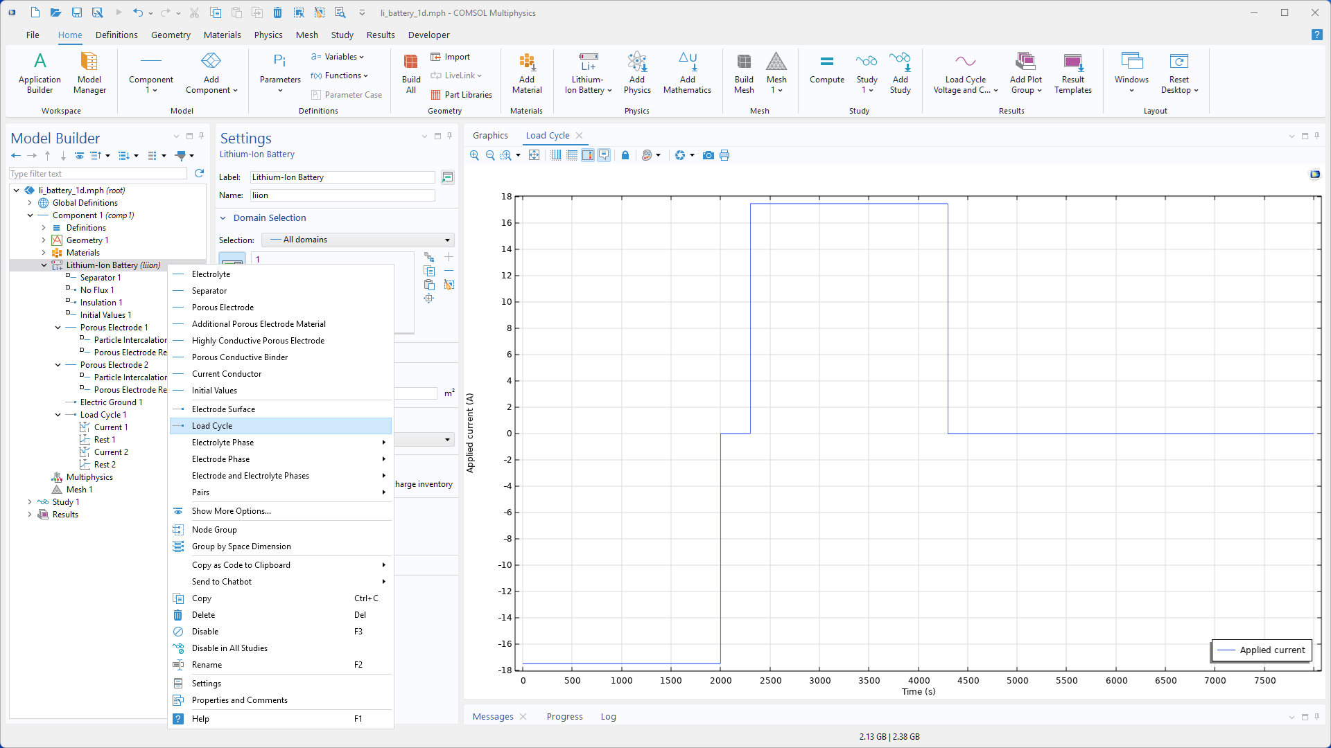 The Load Cycle feature can be found as a boundary condition by right-clicking on the Lithium-Ion Battery and Battery with Binary Electrolyte interfaces or selecting from the ribbon menu.
What the Load Cycle Feature Offers
In the Load Cycle Settings window, the load type can be selected. In the Load Type section, you can choose between Galvanostatic, Potentiostatic, or a combination of both, as shown in the screenshot below. Selecting either galvanostatic or potentiostatic limits the available operation modes to Current and C-rate, or to Voltage, respectively, along with the Rest and Subloop child nodes. Choosing the combined option Potentiostatic and galvanostatic enables access to all modes, including power.
Transitions between added operation modes can be based on multiple criteria, including elapsed time, cutoff values (such as voltage or current), or any user-defined expression. If the Use elapsed time only option is selected at the top level, transitions are restricted to elapsed-time-based (explicit) switching. Otherwise, additional options are also available to control transitions between modes.
The Load Cycle Settings window includes options for terminating the load cycle, such as limits based on total cycling time, number of cycles, voltage thresholds, or user-defined criteria. This built-in functionality allows users to define the end of cycling without manually introducing variables or adding stop conditions in the solver configuration. These conditions can be selected from the Cycling Stop Condition drop-down menu in the Load Cycle Settings window.
The settings also allow users to enable built-in global probes, which automatically monitor voltage and current. Using probes in the model, regardless of the physics involved, offers advantages, such as allowing you to view results without waiting for the simulation to finish, to use probe variables (which are global) in the results section, or to define expressions within the model. In battery modeling, in particular, monitoring voltage and current during the simulation is highly recommended, as it helps understand how the battery behaves under the load cycle and assists with troubleshooting.
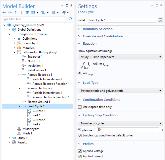 The Load Cycle Settings window shows the load type selection, the option to restrict the continuation method to elapsed time only, and settings for cycling stop conditions and voltage and current probes.
Using the Load Cycle Feature
Any load profile can be defined by specifying its steps, the characteristics of each step, the transitions between them, and the conditions for stopping the cycling sequence. With the Load Cycle node added to the Lithium-Ion Battery interface (or to any Electrochemistry interface) and the load type set in the Load Cycle Settings window, construction of the load profile begins by adding the profile steps in sequence: right-click the node and add the corresponding step. Once the steps have been added and arranged as desired, each step can be customized by applying a constant value or assigning a function to capture that step’s characteristics. The input type for each step can be selected in the corresponding Settings window from a drop-down menu, with options for value, function, or step sequence to define the input values. Each step of the load cycle is followed by the next when the switching condition, defined through the Continuation Condition, is met and enforced using solver events.
Although using functions to define the load profile was discussed in Part 1, incorporating them into this event-based framework improves numerical stability when the load is applied to the model since function smoothing is not required. Alternatively, you can use a step sequence, which enables importing or locally define a table of times at which the set value is updated. This option is particularly useful when importing a user-defined load profile, such as a drive cycle, from a text file into COMSOL®. The screenshots below represent two different load profile examples, each constructed with different steps and input types.
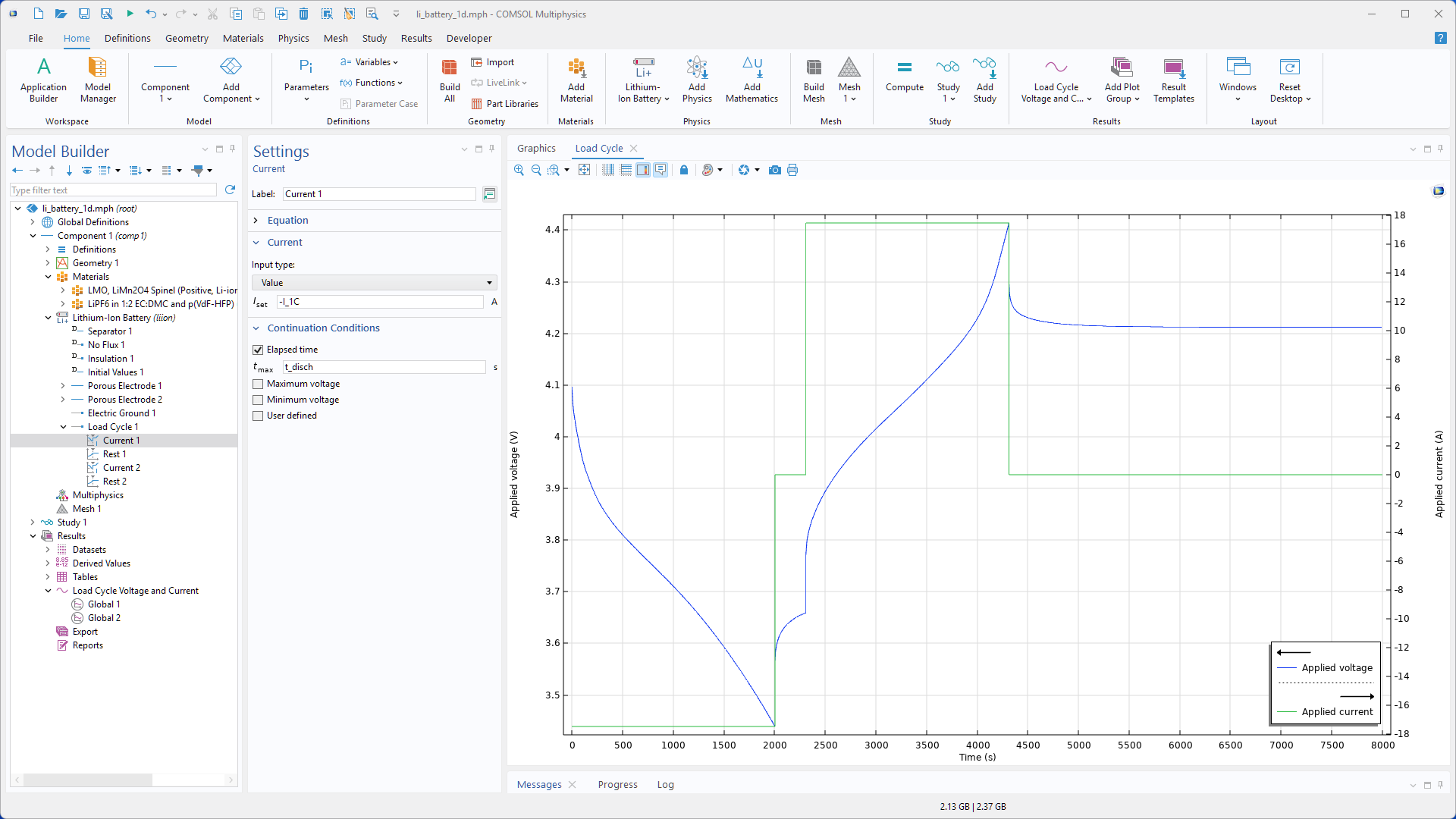 A 1C constant-current charge and discharge profile with known durations, with a rest period in between ad final rest step is defined using the Load Cycle feature.
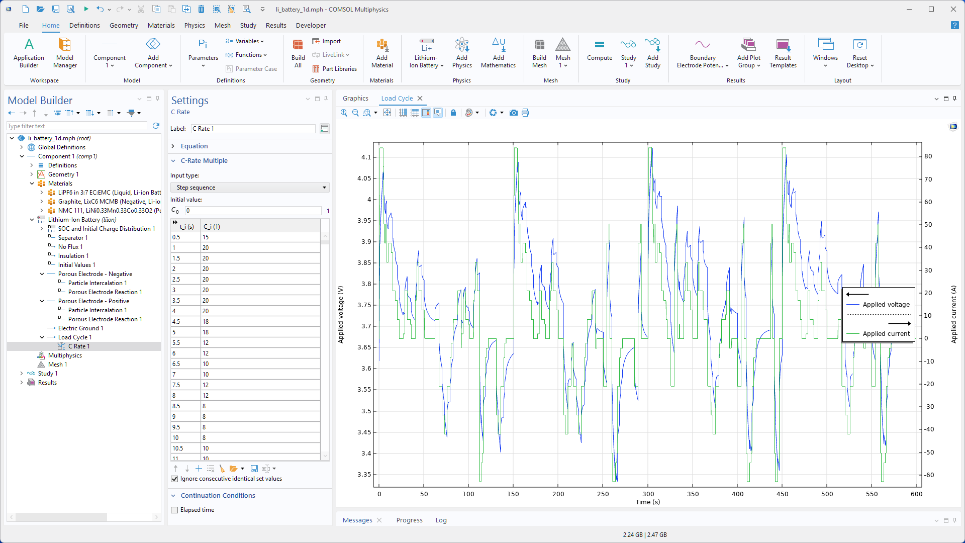 A drive-cycle based on a table of time versus C-rate is defined by selecting “Step sequence” as the input type for the C-rate.
To cover scenarios that require a nested loop within a main sequence, the Subloop child node can be added. This feature is only accessible if Use elapsed time only has not been selected in the Load Cycle settings. The Subloop contains its own nodes for different modes of operation, similar to the main sequence, representing a loop within the overall protocol. The Subloop iterates over these modes, and its duration is controlled by a selected break condition. This condition can be based on elapsed time, number of cycles, or a user-defined criterion. Once the condition is met, the simulation returns to the main sequence or, if the subloop is the final step, proceeds to the first node under the Load Cycle node. The screenshot below shows a simple profile with a subloop. Such a profile can be easily extended to include multiple subloops with completely different modes of operation and termination criteria.
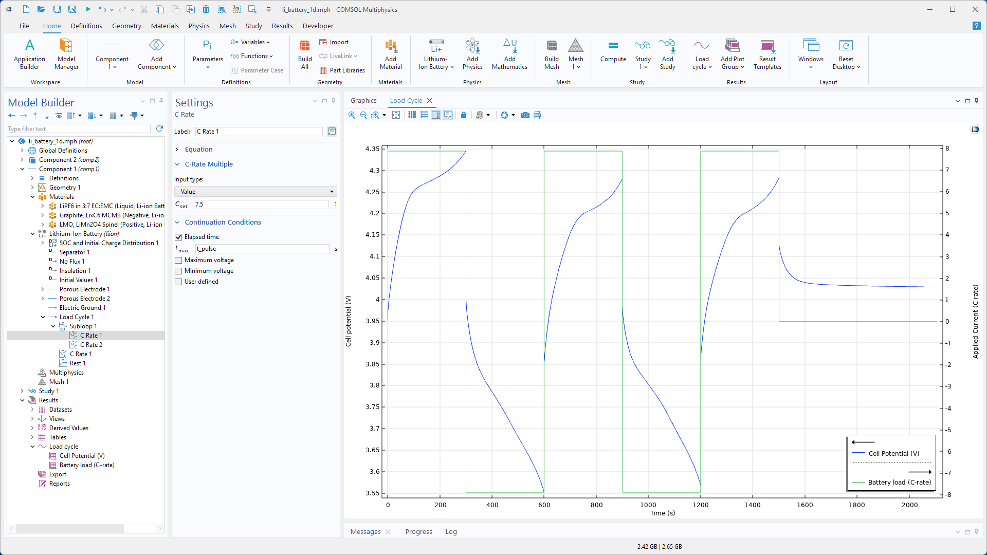 The Subloop feature defines a profile consisting of two cycles of charge and discharge pulses, followed by a charge pulse and a rest period.
Conclusion
Although all the methods for defining load cycles covered in the Part 1 remain valid, the Load Cycle feature introduced in version 6.4 offers a more straightforward and numerically robust approach that also supports complex, custom profiles. Key aspects of this functionality have been covered in this blog, and users can now start using it in their battery simulations. Most examples in the Application Library have been updated to use this feature and can serve as demonstrations of different scenarios implemented with it.


Comments (0)