
In an earlier blog post, we considered the computation of acoustic radiation force using a perturbation approach. This method has the advantage of being both robust and fast; however, it relies heavily on the theoretical evaluation of correct perturbation terms. The idea behind the method presented here is to solve the problem by deducing the radiation force from the solution of the full nonlinear set of Navier-Stokes equations, interacting with a solid, elastic microparticle.
Fluid-Structure Interaction (FSI) Formulation
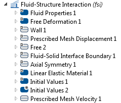
The problem that we want to solve involves the motion of a fluid due to the acoustic wave, which in turn exerts force on a solid particle. The particle responds to the applied force by deformation and net motion and also applies reaction forces on the fluid. This means that in addition to solving the equations describing the fluid dynamics, you would also need to account for the deformation of the particle and the resulting deformation of the space occupied by the fluid. The pre-built Fluid-Structure Interaction physics interface in COMSOL Multiphysics® software allows you to solve this problem by coupling fluid flow, structural stress analysis, and mesh deformation.
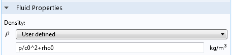
The acoustic radiation force is a nonlinear effect, where the nonlinearity is inherent to the flow and stems from the convective term (\mathbf u \cdot \nabla )\mathbf u in the Navier-Stokes equation rather than from the material nonlinearity. To support acoustic waves, the fluid has to be compressible. The fluid compressibility can be introduced by modifying the constitutive relation of the fluid. We assume a linear elastic fluid where p = c_0^2(\rho-\rho_0) and, for water, we put c_0 = 1500 m/s and \rho_0 = 1000 kg/m3. Because we initially want to compare the method with classical, analytical models that neglect the effect of viscosity, we assume an arbitrary, small viscosity value.
The acoustic radiation force is much higher in the standing wave fields, and most practical applications utilizing this effect involve standing waves. Let us examine this case.
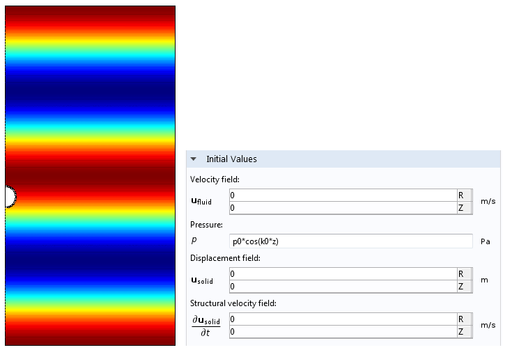
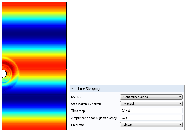
Because the problem is nonlinear, it must be solved in the time domain. Since the solution can be quite time consuming, we will solve it in a 2D axisymmetric geometry. To create a standing wave in a time-dependent solution, we consider a resonant box two wavelengths high and initiate the standing wave by setting up the corresponding initial conditions. For example, in a box two wavelengths high, the standing wave solution would be p(r,z,t) = p_0 cos(k_0 z) cos(\omega t) and, at the time t= 0 , the initial conditions should read p(r,z,t=0) = p_0 cos(k_0 z) and \mathbf u(r,z,t=0) = 0. This is illustrated below for a simulation box that is 3 mm high and has a wavelength of \lambda = 1.5 mm (the corresponding frequency is 1 MHz).
As noted in the previous blog post, we expect the nonlinear force term to be a few orders of magnitude smaller than the linear force, such that the particle will appear to be bouncing up and down in the acoustic field. However, every time the particle moves, it will go a little further in one direction than the other. This is a result of the nonlinear force component that does not change its direction when the field changes its sign. Because the nonlinear force is so small, it is very hard to extract the value of the nonlinear force from the time-domain solution, unless a very simple trick is used.
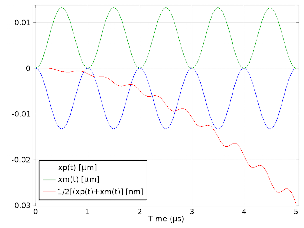
The essence of this trick is to utilize the very fact that the nonlinear force does not change direction when the excitation changes sign. Let us denote x_\textrm p (t) as the average displacement of the particle obtained when p_0 is positive and x_\textrm m (t) when p_0 is negative. The nonlinear displacement component will be given by the combination of the two, x_\textrm{nl}(t) = 1/2 \left [ x_\textrm p (t) +x_\textrm m (t) \right]. This method was first used here. The solution corresponding to the pressure amplitude of 0.1 MPa and a nylon particle of 100-μm radius is depicted in the plot below. You can see that x_\textrm p (t) and x_\textrm m (t) have opposite signs and otherwise appear identical; however, their sum is non-zero, albeit very small in comparison.
Here, the particle is shown in motion.
Notes on Implementation in COMSOL Multiphysics® Software
The method outlined above considers nonlinear acoustic phenomena. Therefore, the usual rules of acoustic modeling apply. They are:
- The mesh has to be sufficiently fine to resolve the shortest wavelength. Here, the basic wavelength is that of the externally imposed standing wave. Shorter wavelengths, however, are produced by the particle vibrating at its resonant frequency. These wavelengths will be captured by the model because it is solved in the time domain.
- A suitable time progression method when resolving wave phenomena in COMSOL Multiphysics is the generalized alpha method. To make sure that the solution is stable, a Courant–Friedrichs–Lewy (CFL) criterion has to be manually imposed by setting a manual step size with \delta t < 0.5\ h_\textrm{min} / c_0.
Postprocessing
The last step of the analysis is computing the force from the average nonlinear displacement given by the finite element model. We can observe the effect of the acoustic radiation force as a small offset of the displacement from the otherwise perfect oscillatory motion of the particle. Judging by the difference in the computed linear and nonlinear components of the displacements, the difference in force components is about three orders of magnitude. So, the effect of the acoustic radiation force is negligible during one acoustic cycle and, to evaluate it correctly, around five to ten acoustic cycles must be computed.
With this data, we can export the results to Excel® spreadsheet software and find the average acceleration by fitting a second-degree polynomial to the displacement curve and computing the force as F = m \ddot x_\textrm{nl}. The graph below shows the results of such an analysis.
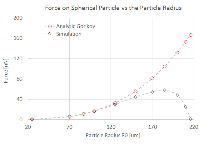
Here, the maximum force at a λ/8 distance from the pressure node of the standing wave is evaluated as a function of the particle’s radius. A good agreement is obtained in the limit of the small particle k_0R_0 \ll 1 for which the analytical model is valid, and the deviation appears to increase as we depart from this limit.
Conclusion
We have outlined a direct method for evaluating nonlinear acoustic radiation force. The same approach can be applied to other nonlinear acoustic effects such as acoustic streaming. The advantage of this method is that it does not rely on any theoretical models (e.g., the perturbation method) to express the nonlinear terms. Note that because the fluid-structure interaction approach requires the model to be solved in the time domain, it is much slower than the perturbation method.
Other Posts in This Series
Excel is a registered trademark of Microsoft Corporation in the United States and/or other countries.


Comments (3)
Niccolò Rondelli
June 1, 2016Is there any possibility to have the guideline for this model or the COMSOL file?
Ulrik Fallrø
January 19, 2018I would also like to see giudelines for modeling if this is possible.
Guido Spinola Durante
November 20, 2019Dear Prof. Grinenko,
I have found most interesting your Comsol blogs on acoustic radiation
https://www.comsol.com/blogs/how-to-compute-the-acoustic-radiation-force/
https://www.comsol.com/blogs/direct-fsi-approach-to-computing-the-acoustic-radiation-force/
Could you explain which conditions you applied to compute Gor’Kov analytic radiation force versus particle size?
Why are the graphs not same in the two different blogs?
Best regards,
Guido Spinola Durante