
There are various ways of handling interactions between fluids and solids in the COMSOL® software. You can, for example, explicitly model the fluid using the full Navier-Stokes equations for the pressure and fluid velocity fields. Although that can be a very accurate approach, it’s much more expensive than is needed for certain types of Fluid-Structure Interaction (FSI) problems. Here, we’ll introduce a method for modeling enclosed volumes containing incompressible fluids, under the additional assumption that the momentum and energy transfer via the fluid is small.
Editor’s note: At the time when this blog post was written, there was no built-in functionality for computing fluid loads in enclosed cavities. The Enclosed Cavity feature was introduced in version 6.2 of COMSOL Multiphysics for doing just that.
Modeling an Enclosed Volume of Fluid
Let’s take a look at an existing example, a model of the compression of a hyperelastic seal. This example considers the cross section of a soft rubber seal as it is compressed. The fluid enclosed in the cavity is air. The example computes the compressive force, and compares the result of including the effect of the compressible air within the seal with the result of not including it.
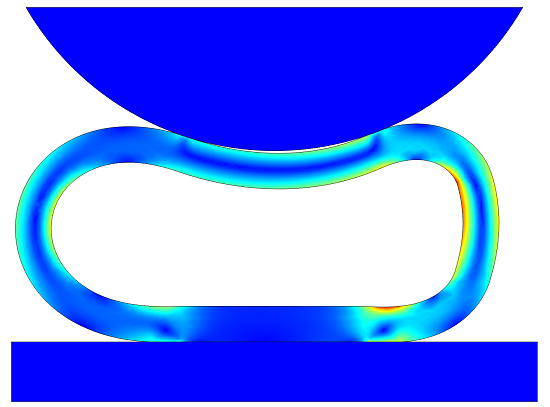
Compression of a soft rubber seal. The stress and deformed shape are shown. Various ways of modeling the air inside of the seal are considered.
The existing model treats the air as a compressible fluid and computes the change in pressure p in the interior of the cavity as a function of the change in the cross-sectional area A of this two-dimensional example. Next, let’s take a look at how this is done. The air is treated as an ideal gas under adiabatic compression, which gives the pressure-density relation:
So to compute the change in pressure, we only need to know the change in area. The original area and pressure are both known, as well as the ratio of specific heats, \gamma. But how do we compute the cross-sectional area? The area is described by a region that we do not even want to include in our model. We can use Gauss’ theorem and convert an area integral to a boundary integral:
Where x is the x-coordinate of the deformed configuration of the seal, and n_x is the x-component of the outward facing normal vector to the boundary, also in the deformed configuration, thus giving us the enclosed area within the seal. This is done via an Integration Coupling Operator, called AreaInt, defined over the complete interior boundary of the enclosed volume. A variable, EnclosedArea, defined on the “Entire model”, defines the deformed area.
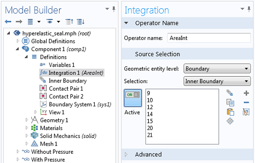
The area integral is defined over the inner boundaries of the seal.
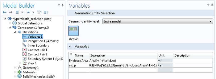
The definition of the variables that defines the enclosed area and internal pressure, respectively. The negative sign must be used to compute the area since the normal to the solid is directed into the cavity.
The computed deformed area is used to determine the change in the internal pressure of the seal as it is deformed. This computed differential pressure is computed and applied as a load to the interior of the seal. To see the complete implementation of the above method, please look through the existing documentation for this model.
Considering an Incompressible Fluid
The above approach assumes that the fluid is compressible and that the internal pressure of the seal is a function of the change in area. But what if the fluid is incompressible? Let’s suppose that, instead of compressible air inside the seal, we are dealing with a bladder filled with water — which is very nearly incompressible. Then the enclosed area cannot change as the structure is deformed, and the above approach will not work. Therefore, we need an alternative.
We will introduce one more equation into this model, via the Global Equations feature added to the Solid Mechanics interface, to solve for the pressure within the fluid such that the volume doesn’t change. Let’s take a look at the interface:
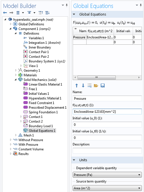
The settings for the additional global equation. You will need to enable the Advanced Physics Options to view this feature.
The above screenshot shows the Global Equation settings for the additional variable, Pressure. The equation being satisfied is that the variable, EnclosedArea, equals the initial area, 123.63mm2. That is, the variable Pressure takes on whatever value is needed so that the enclosed area of the deformed shape equals the initial area. The variable Pressure is then applied to the interior of the seal via the Boundary Load feature, and the model is re-solved.
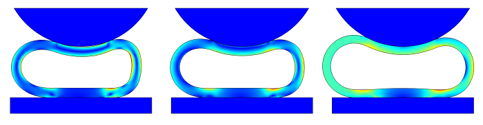
Comparison of solutions. No internal pressure (left), compressible air (center), and an incompressible fluid (right).
Concluding Remarks
In this example, we have introduced a technique for modeling the interaction of an incompressible fluid and a deformable solid. By adding a global equation, we introduce one additional variable to the model that solves for the applied pressure needed to maintain a constant volume. This represents one of the simplest ways of solving a fluid-structure interaction problem.


Comments (4)
Shuai Ge
March 31, 2014Hi Walter,
Thanks for posting this thread. It is very helpful for my simulation work. Following the guidelines, I did the simulation of incompressible fluid successfully in 2D with COMSOL4.2a. But when I try to translate this technique into 3D model, I get the following error. Will you have any suggestions on my debugging process? Thanks a lot!
****************************************
Failed to find a solution.
Singular matrix.
There are 1 void equations (empty rows in matrix) for the variable comp1.Inner_pressure.
at coordinates: (0,0,0), …
Returned solution is not converged.
****************************************
Walter Frei
April 2, 2014 COMSOL EmployeeHello Shuai,
The issue here is likely that you would want to use a fully coupled direct solver, for the reasons outlined here:
http://www.comsol.com/blogs/improving-convergence-multiphysics-problems/
If this does not address the issue, you should contact the COMSOL Support Team.
Shuai Ge
April 7, 2014Hey Walter,
Thanks for your response. I checked the solver, it is using fully coupled direct solver by default. I’ve tried to ramp up the load to eliminate any large nonlinear problem, but it is not fixed still. I’ll contact the support. Followed is the thread link I posted with the model file attached, only if you could take a look. Thanks a lot!
Best,
Shuai
http://www.comsol.com/community/forums/general/thread/43551/
Walter Frei
February 5, 2021 COMSOL EmployeeHello Readers,
For additional information regarding solving models with these kinds of coupling operators, see also:
https://www.comsol.com/blogs/accelerating-model-convergence-with-symbolic-differentiation/