Results & Visualization Blog Posts
Postprocessing Local Data Using Component Coupling
Derive numerical values. Create new coordinate systems. Link different components in the same model. How can you accomplish all of these tasks? By using Component Coupling operators.
Useful Tools for Postprocessing in COMSOL Multiphysics
Layering plots; style inheritance; enabling and disabling grids, axes, and legends; showing mesh plots, and more: We go over some useful tools for postprocessing your simulation results.
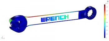
Using Deformations to Visualize Physical Motion
Postprocessing and visualization can help enhance your understanding of simulation results, and using plots to illustrate physical motion allows you to put everything into perspective.
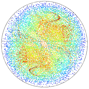
Application-Specific: Polar, Far-Field, and Particle Tracing Plots
When postprocessing your electromagnetics models, you can use polar, far-field, and particle tracing plots to effectively display your results. Learn how to use these 3 plot types here.
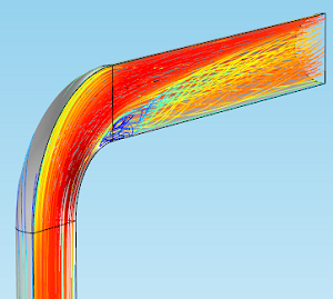
Visualizing Fluid Flow with Streamline Plots
As part of our blog series on postprocessing, we demonstrate the use of streamlines to visually describe fluid flow in your simulations. Learn how with an example of flow through a pipe elbow.
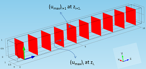
Maximum Evaluations on Parallel Sections
Postprocessing trick: You can evaluate and plot the maximum, minimum, average, or integration value of any variable at various parallel sections along the axial coordinate of your model.
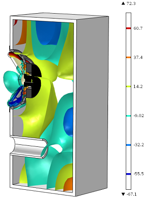
Making Waves with Contour and Isosurface Plots
In this installment of our blog series on postprocessing your simulation results, learn how to use contour and isosurface plots to show quantities on a series of lines or surfaces.
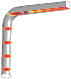
Using Slice Plots to Show Results on Cross-Sectional Surfaces
In this installment of our blog series on postprocessing your simulation results, we demonstrate slice plots, an easy way to visualize physics behavior on many different parts of your model.
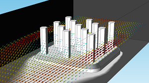
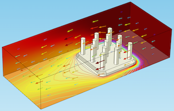
How to Get the Most out of Arrow Plots in COMSOL Multiphysics
What are arrow plots and why are they useful? We answer these questions and demonstrate how to use this feature in this installment of our postprocessing series.
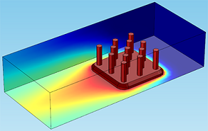
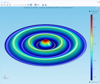
Surface, Volume, and Line Plots: Visualizing Results on a Heat Sink
3 of the most common plot types used in postprocessing: surface, volume, and line plots. Learn how to use these plot types for your simulation results and when to use each option.
Combining Parallel Slices to Create an Animation
Want to animate how your 3D steady-state model’s solution is changing along a certain direction? You can do so by combining parallel slices. We demonstrate the 3-step process…
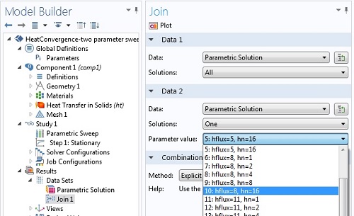
Solution Joining for Parametric, Eigenfrequency, and Time-Dependent Problems
In a follow-up to a previous blog post, we demonstrate how to use the Join feature in the context of 4 types of problems: parametric, eigenfrequency, frequency domain, and time dependent.