
Over half a century ago, Mark Kac gave an interesting lecture on a question that he had heard from Professor Bochner ten years earlier: “Can one hear the shape of a drum?” He focused on the (then undetermined) uniqueness of the set of eigenvalues given the shape of a vibrating membrane. The eigenvalue problem has since been solved and here we explore the “hearing” part of the question by considering some interesting physical effects.
The Original Eigenvalue Problem: The Quest for Isospectral Drums
Consider a drum head constructed by stretching a membrane over a stiff frame that encloses a flat 2D domain. The vibration of the membrane is described by the wave equation (Helmholtz equation) with the Dirichlet boundary condition at the periphery of the domain where the membrane is constrained by the stiff frame. In this case, there is a set of discrete solutions to the wave equation, called normal modes or eigenmodes, each of which vibrates at a characteristic frequency, called eigenfrequencies.
The lowest eigenfrequency defines the fundamental tone, which for instance could be concert pitch A (440 Hz). The set of higher eigenfrequencies, or overtones in musical terms, gives rise to the tone color or timbre of the vibrating membrane. Kac’s lecture drew our attention to the eigenfrequencies: Is it possible to construct two drum heads with different shapes that share a set of eigenfrequencies? The idea was that if the two drums have an identical set of eigenfrequencies (being isospectral), then they would have the same timbre and sound the same to the ear, even though their shapes are different.
Kac commented on the asymptotic behavior of the eigenfrequencies in the limit of very high frequencies and made connections to various branches of physics and mathematics to provide a ground for intuitive understanding. The uniqueness question (in 2D flat space) remained unsolved until over two decades later when Gordon, Webb, and Wolpert finally constructed two polygons with an identical set of eigenvalues (see “One cannot hear the shape of a drum” and “Isospectral plane domains and surfaces via Riemannian orbifolds“).
The eigenvalues of the two polygons can be computed numerically, which is shown in this Isospectral Drums model in our Model Gallery.
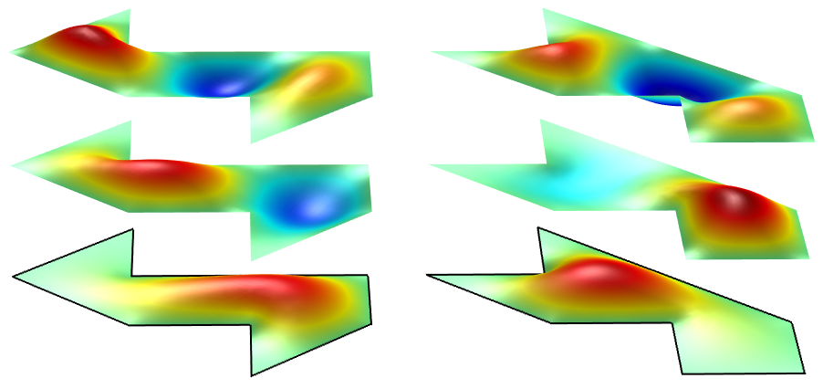
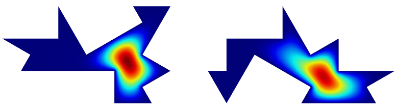
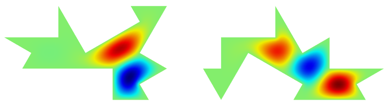
The image below shows the first three normal modes of the two polygons that share the same set of eigenfrequencies:
In Gordon and Webb’s easy-to-read introductory article on this subject (“You can’t hear the shape of a drum”, American Scientist, vol. 84 (1996), pp. 46–55), they commented that such isospectral drums with different shapes are expected to be the exception, not the rule. In other words, they expected that, in general, one can hear the shape of a drum, unless the shape of the drum is specially constructed to be isospectral with another shape, like the two polygons depicted above.
In the following discussion, we will take a closer look at such special shapes by considering various physical mechanisms involved in the sound production and detection. We will find that when we include relevant physical effects, we actually can tell two drums apart by the sound, even if they are specially constructed to share the same set of eigenfrequencies.
The Excitation of the Membrane Motion
The first effect we will examine is the excitation of the vibrational modes in the membrane. Since the timbre is determined by the set of relative amplitudes of the normal modes, it is not enough to just have an identical set of eigenfrequencies for the two drums to sound the same. They also need to have the same relative amplitude for each eigenmode, which may not be trivial to achieve.
Let’s take, for example, the same two polygonal drums from above and hit them with a drum stick at a few arbitrary places, one at a time, as such:
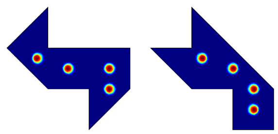
Each location of striking is somewhere in the middle of the drum, where a child may instinctively choose to hit if given such a drum and a drum stick. We use COMSOL Multiphysics simulation software to calculate the frequency response of each of the locations and plot the results in the graphs below.
We first focus on just one drum, say, the one on the left. Here is a plot showing the left drum’s frequency response:
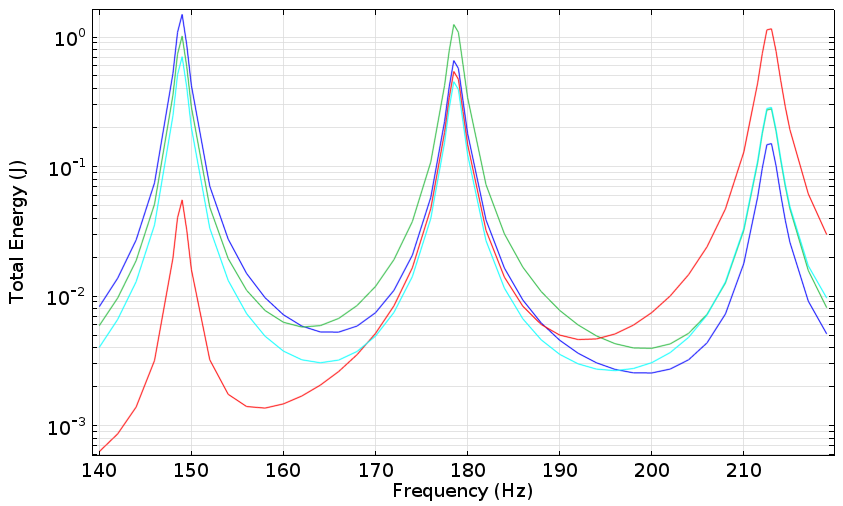
As we hinted at earlier, the drum sounds differently depending on the location where it is struck by the drum stick. We see different energy distribution among the first three eigenmodes, which will result in different timbre. This is, of course, a well-known fact to percussionists and is the result of the same principle that enables a single bell to ring in two distinct tones, as demonstrated by this ancient set of bells from over two thousand years ago.
Now we know we can’t even make one drum sound the same unless we have a perfect aim of the drum stick. Is there any hope that we can make the two different drums sound the same?
In the graph below, we’ve added the frequency response of the second drum (the dashed curves). As we examine the graph, it becomes evident that none of the dashed curves match the solid curves in all three of the eigenmodes. In other words, the two drums do sound differently, even though they are isospectral, sharing the same set of eigenfrequencies.
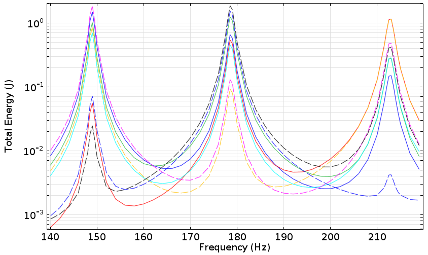
Of course, we haven’t done an exhaustive search of all the possible combinations of striking locations. However, this simple example illustrates that it is not an easy job to make the drums sound the same, due to the different coupling strengths of energy from the drum stick to the various vibrational modes of the membrane.
Homophonic Drums
The magic of mathematics never ceases to amaze us. Not long after the two isospectral polygons were published, Buser, Conway, Doyle, and Semmler constructed a pair of domains that are not only isospectral (sharing the same set of eigenfrequencies), but also homophonic: having a special point in the domain such that “corresponding normalized Dirichlet eigenfunctions take equal values at the distinguished points” (“Some planar isospectral domains“). In other words, if the special point of each drum is hit by a drum stick, then each corresponding pair of eigenmodes of the two drums will be excited with the same amplitude and the two drums will sound the same.
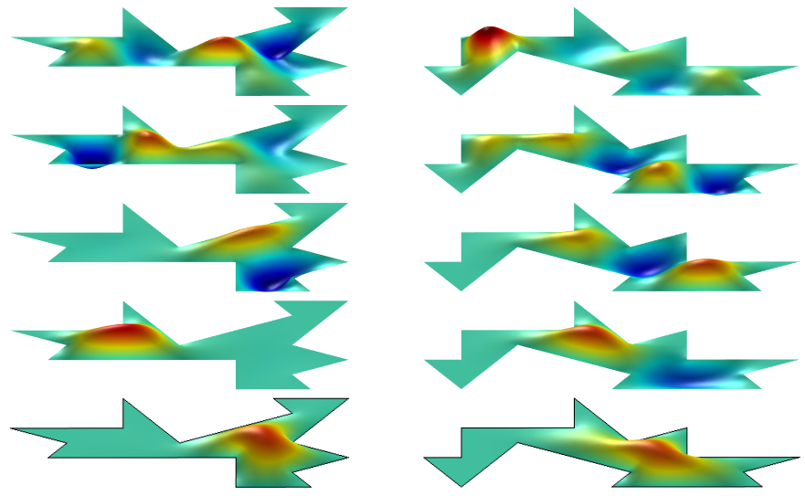
Shown below are the first few normal mode shapes computed numerically:
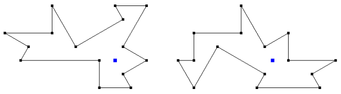
The special point of each domain is marked with a blue square in the schematic below:
In the following graph, we plot the computed frequency response of the two drums to a narrow Gaussian area load centered on each of the special points:
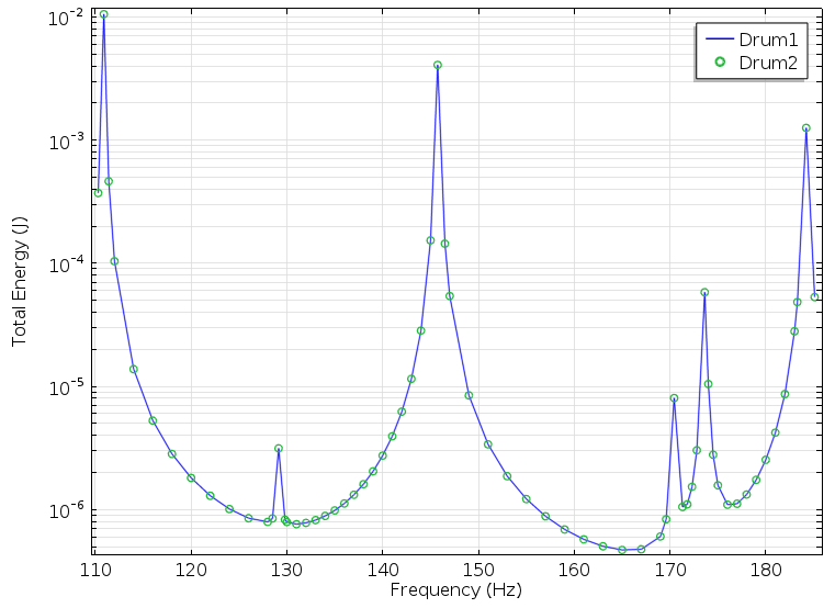
Isn’t it amazing how well the two frequency response curves (solid blue curve and green circles) lie on top of each other? With such a perfectly matched vibrational energy spectrum, wouldn’t the two drums sound exactly the same? Let’s continue our journey to explore more physical effects and find out.
The Propagation of Sound Waves in Different Directions
Our ears do not sense the vibration of the membrane directly. Rather, the sensing is mediated by the acoustic wave in the air. Let’s set up the two homophonic drums outdoors, where the sound is allowed to propagate away from the drums without significant reflection. In this case, we can easily compute the frequency spectrum of the sound wave using COMSOL Multiphysics to find out what we really hear with our ears.
Let’s take a look at the three vibrational modes with the highest energies at about 111, 146, and 184 Hz as shown in the spectral graph above. For convenience, we will call them the first, second, and third mode, with the understanding that there are other modes in between being neglected since they are much less energetic.
The polar graph below compares the computed sound pressure level (in dB) in the plane of each of the two drums, a few meters away from each drum.
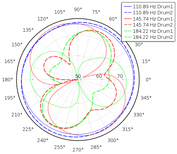
We see that the sound pressure field produced by the first mode is more or less independent of direction (solid and dashed blue curves). This is not surprising, since the mode shape of each drum looks pretty much like a monopole source:
On the other hand, the directionality of the sound field from the second or the third mode of each of the drums is quite pronounced and also quite different between the two drums. For example, for the second mode, the sound field from Drum 1 looks like a dipole field (solid red curve), while the one from Drum 2 is more complex (dashed red curve). This observation again matches what we see in the mode shapes of the two drums:
What really determines the perceived timbre is the ratio of the amplitudes of the higher modes (the overtones) to the lowest mode (the fundamental tone). So, in the next graph, we plot the amplitude ratios of the second and the third modes to the first mode, at a sampling of directions:
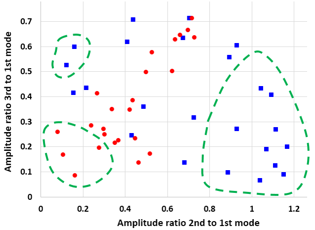
The blue square points are from Drum 1 and the red round points from Drum 2. The graph can be viewed as a map of timbre — if two points on the graph are near each other, then they sound similar; on the other hand, if two points on the graph are far away from each other, then they have very distinct timbre. As qualitatively illustrated by the green dashed boundaries, each drum can produce a range of timbre that the other cannot, in some range of directions.
As long as a listener is allowed to move around each drum, perhaps blindfolded, he or she will hear distinct ranges of timbre that tell the two drums apart. Therefore, even though the two “homophonic” drums share the same energy spectrum in their vibration modes, due to the difference in the mode shape and to the difference in energy transfer to the sound field in the air, the acoustic energy spectrum in some range of directions can be quite different. This is what would cause the two drums to sound differently to our ears.
The Shift of Eigenfrequencies Due to Air Loading
In the previous analysis, we ignored the reaction force acted on the membrane by the air, the so-called air loading effect. It turns out that this effect is very significant for a real drum, since, after all, the entire area of the membrane participates in the pushing and pulling of the air around it.
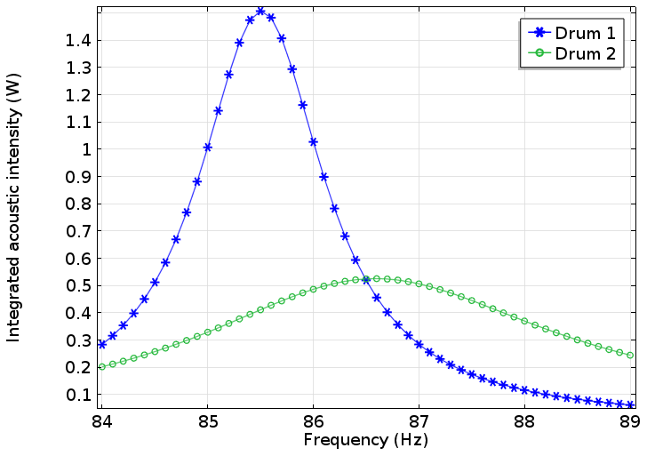
We can simulate this effect using the Acoustic-Structure Boundary Multiphysics coupling feature of COMSOL Multiphysics. We find, for example, that the eigenfrequency of the second mode that we were discussing shifts from 146 Hz down to about 86 Hz. In addition, the magnitudes of shift of the two drums are different. The eigenfrequency of one drum was shifted down to 85.6 Hz, while the one of the other drum shifted to 86.8 Hz. This difference causes a pitch difference of about 23 cents, which is very audible in a side-by-side comparison.
Therefore, not only do the two drums differ in timbre (in some range of directions), they also differ in absolute pitch when we take the air loading effect into account.
The graph below shows the frequency response of the two drums around this mode. The difference in the resonant frequency is clearly seen, as well as the difference in the width of the resonance. There should be no doubt in our mind that with such different frequency responses, the two drums will produce easily distinguishable sounds.
Concluding Remarks
It is a great achievement in mathematics to invent the isospectral drums that share the same set of eigenfrequencies and the homophonic drums that share the same power spectrum of the vibrational modes when excited at a special point. However, these phenomena only happen in vacuum, where there is no sound. Once we put the drums to test in air, they start to sound differently due to the air loading effect and the directionality of the energy transfer from the membrane to the sound wave.
In his lecture, Kac told the early 20th-century story of Lorentz calling for mathematicians’ attention to the eigenvalue problem involved in the theory of black body radiation and Weyl answering the call with the proof of the theorem of the asymptotic behavior of eigenvalues at very high frequencies.
Here, we could use the help of our mathematician friends again, even though the subject matter may not be as grand as black body radiation and quantum mechanics. Is it possible to construct homophonic drums with different shapes that sound the same when including directionality and air loading effects? It may be possible to pose this as an optimization problem to solve numerically for a solution with a finite set of audible frequencies.
However, the computation cost will be high and the result will be approximate. An elegant analytical solution similar to those shown in the papers mentioned above would be much nicer. I hope this will arouse the interest of mathematicians who are reading.


Comments (3)
Isaac Snitkoff
May 4, 2020Are you able to provide the files you used to get these models? I am trying to replicate and am having trouble.
Brianne Christopher
May 5, 2020 COMSOL EmployeeHello Isaac,
Thank you for your comment.
For questions related to your modeling, please contact our Support team.
Online Support Center: https://www.comsol.com/support
Email: support@comsol.com
Tina Sager
July 28, 2022How can I simulate the vibrational modes of a membrane when it is struck at different locations?