Learning Center

Efficient Solving of MHD Models

---

The final stage of setting up a magnetohydrodynamics (MHD) model is configuring the solver to run efficiently and return accurate results. In this part of the course, we will discuss techniques for solving highly nonlinear high Hartmann number models in the COMSOL Multiphysics^® software, including what adjustments to make to improve the speed and accuracy of the solvers.

Solving for High Hartmann Numbers

At high Hartmann numbers, the problem can be very difficult to solve, as the Lorentz force from a large magnetic field causes a highly nonlinear problem that is difficult to converge. The standard method for solving these highly nonlinear problems is to apply load ramping, which slowly increases the nonlinearity of the problem, working up to the solution of the true system. The theory behind load ramping has been discussed previously here.

For high Hartmann numbers that are difficult to solve, it is then possible to solve a version of the model with a lower Hartmann number and then slowly increase the Hartmann number up to its true value.

This requires defining a sweep over the Hartmann number in the model. As the Hartmann number is a measure of the system rather than an input, in order to change the system by changing , it is first necessary to express one of the inputs that contributes to the Hartmann number — , the magnetic field; , the fluid's electrical conductivity; or , the dynamic viscosity of the fluid — as a function of the parameter for the Hartmann number. When there is a uniform background magnetic field in the system, the most common choice of input to vary is this background magnetic field.

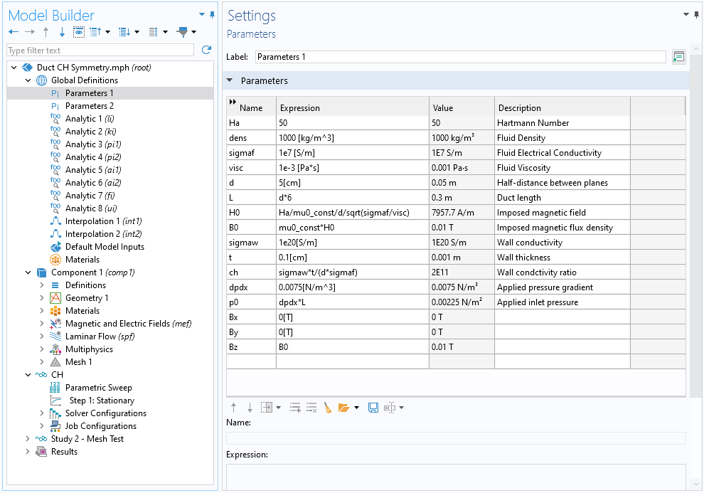The Parameters Settings window with the names, expressions, values, and descriptions for the needed parameters. Calculating the applied background magnetic flux density for a duct flow model from the Hartmann number for load ramping.

There are two possible methods of performing the sweep over , gradually increasing its value.

If the geometry and mesh are independent of the Hartmann number, then an auxiliary sweep can be used. This sweep is enabled as a study extension in the Stationary study step. The auxiliary sweep will automatically use the solution for the previously solved for Hartmann number as the initial condition for the next value that is to be solved for. If the steps between the Hartmann numbers are too large for the solver to converge for the next value of , the sweep will automatically take additional steps in as required to complete the load ramp.

However, if the geometry and mesh are dependent on the Hartmann number, an auxiliary sweep cannot be used, as it cannot adjust the geometry and mesh during the sweep. Instead, it is necessary to use a parametric sweep to sweep over the different values of .

The default settings for Parametric Sweep will not perform load ramping as is swept over. This is because the solver will always use the initial values defined in the Initial Values node as the starting condition for solving when changes. To create a load ramp by using the solution for the previous value of as the next initial value, it is necessary to enable the Reuse solution from previous step checkbox in the Advanced Settings section of the settings for the sweep.

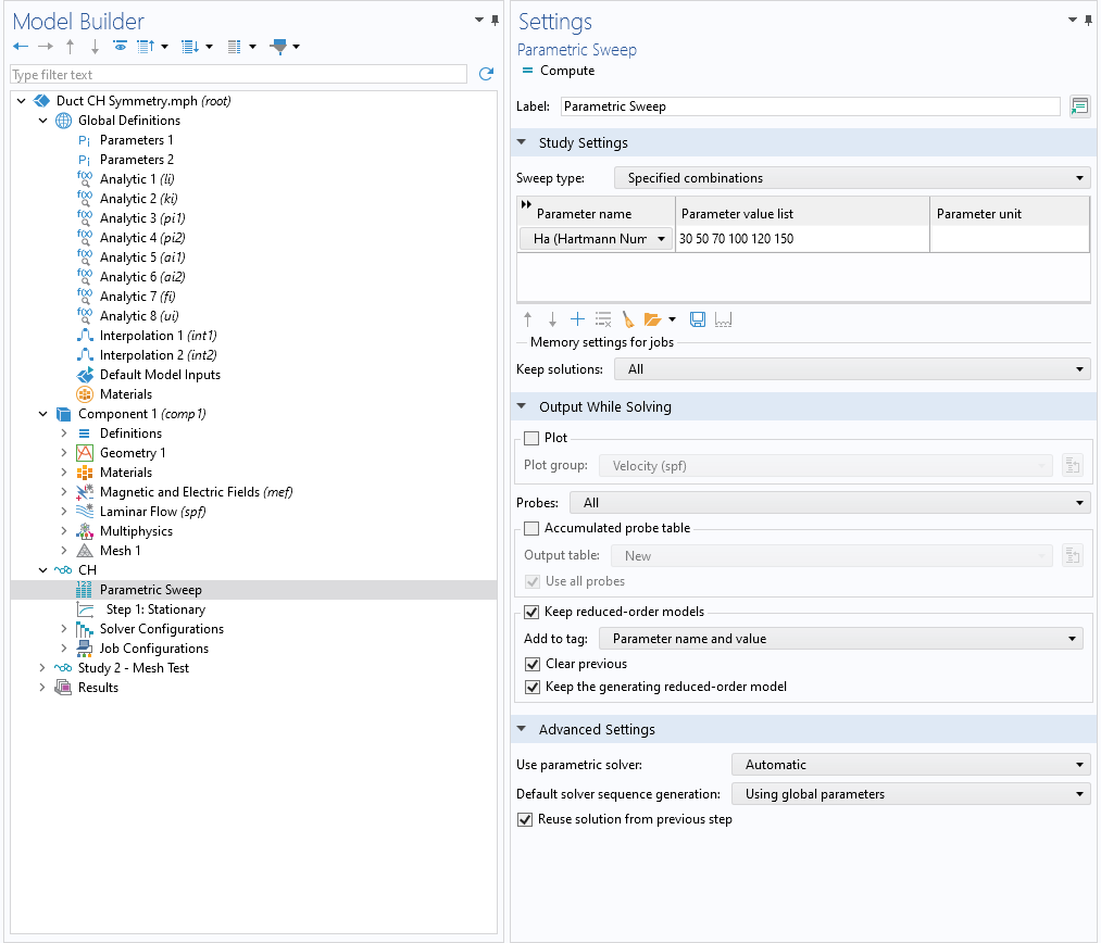The Parametric Sweep Settings window with the parameter values set and the Reuse solution from previous step option enabled. Enabling the option to reuse the solution from the previous step in order to allow the parametric sweep to act as a load ramp for the Hartmann number.

Configuring the Solver

The solver configurations that are automatically generated for the study typically have sufficient solving efficiency, but there are also manual adjustments that can be made to improve solver efficiency and accuracy.

The solver configurationsare automatically generated when a study is run. To access them before a study is run, right-click on the study node and choose either Show Default Solver or Get Initial Value. Using the Get Initial Values step has the advantage of also generating the default plots for the model. The Solver Configurations node can then be inspected.

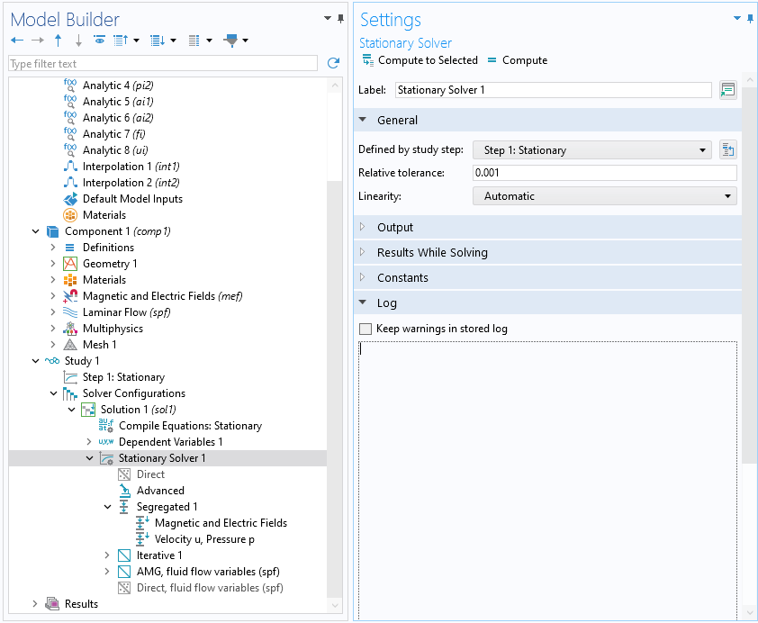The Stationary Solver Settings window with the default settings. The solver configuration generated by default for an MHD model.

There are two approaches to configuring the solver for electromagnetic and fluid flow physics, the fully coupled and segregated approaches. These approaches are discussed in the article Understanding the Fully Coupled vs. Segregated approach and Direct vs. Iterative Linear Solvers.

The fully coupled approach forms a single large system of equations that solves for the electromagnetic and fluid variables and the couplings between them at once, in a single process. The segregated approach divides the full system of equations into smaller subsets and then iterates between solving these. In MHD models, this approach appears as solving first for the electromagnetic fields while fixing the values of u, and then solving for u while fixing the electromagnetic fields. This process repeats until a solution is found. Both of these solver methods have advantages and disadvantages when solving MHD problems.

The segregated approach is generally the default method applied to 3D models. It is more memory light; however, by splitting up the equations, the effects of the couplings between them are suppressed. This has an effect of, for example, suppressing or shifting the positions of the jets. This can be resolved by significantly reducing the tolerance of the solver and increasing the number of iterations allowed, as will be discussed below. The amount the tolerance must be decreased is dependent on the Hartmann number, the fluid velocity, and the material properties of the fluid. As the Hartmann number and fluid velocity increase, the tolerance must be tightened.

The fully coupled approach incorporates all of the coupling terms in every iteration. This means that the nonlinear couplings act more strongly, and an accurate solution is found in a smaller number of iterations. However, this approach can be significantly more memory intense and may not be feasible to use for large 3D models. It is the default approach in 2D models, which are less memory intensive. In 3D, if the default segregated solver fails to converge or generates inaccurate results, switching to the Fully Coupled solver will often resolve the issues without requiring further solver adjustment.

It is recommended to work with the Fully Coupled solver whenever there is sufficient memory available.

Additional Note: If a Segregated solver is required in an MHD model due to it also containing other types of physics, the equivalent technique of using a Fully Coupled solver for the MHD is to modify the Segregated solver steps to solve all dependent variables related to the EM field in the same segregated step as v and p.

After either the Fully Coupled or Segregated solver has been chosen, its efficiency can be improved by utilizing its Stabilization and acceleration settings. CFD modeling commonly uses pseudo time stepping and Anderson acceleration to improve solver convergence. This carries over to MHD modeling.

Pseudo time stepping stabilizes convergence by acting as a form of load ramping. It uses an added time dependency (the pseudo time) to gradually evolve the solution into its steady-state form. The settings allow the CFL number for the pseudo time stepping to be adjusted. The CFL number is a function of the nonlinear error estimate and controls the length of the pseudo time step, which is inversely proportional to the CFL number.

Anderson acceleration means that when solving nonlinear problems with the Newton–Raphson method, the steps taken by the nonlinear solver use information from previous steps rather than just the current step. This provides an acceleration method where oscillations in the convergence of the solver are smoothed out, making the convergence of the solver more efficient.

Pseudo time stepping is more effective at stabilizing convergence when the nonlinear solver is far away from finding the root, whereas Anderson acceleration is more effective when near the root. It is thus possible to use both methods in a model and automatically switch between them when required. This is also controlled by the CFL number, with exchange occurring when it reaches the set CFL threshold.

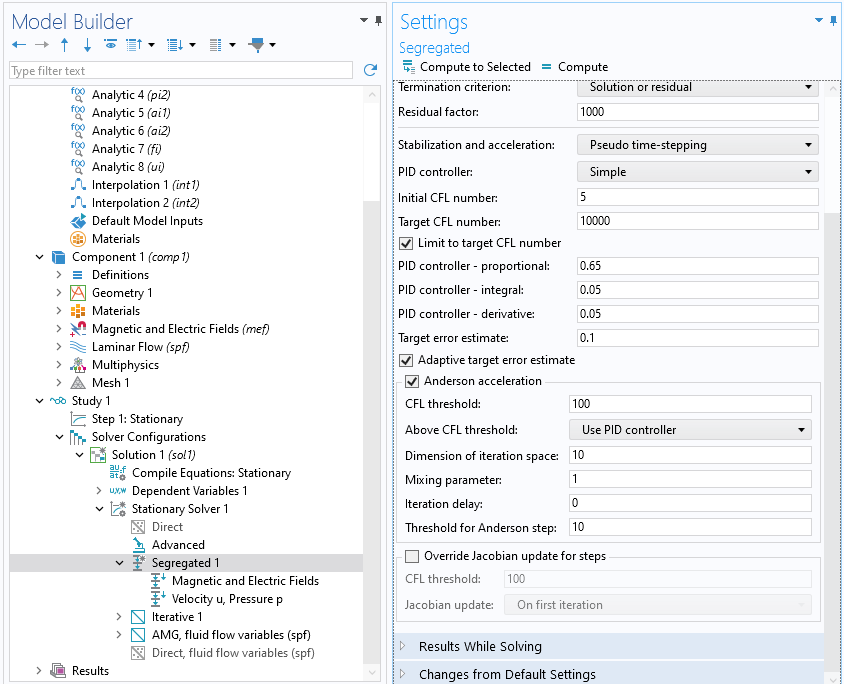The Segregated solver Settings window with Anderson acceleration enabled. Enabling Anderson acceleration in the Segregated solver.

The Fully Coupled solver will often generate an accurate solution to an MHD problem with no adjustments to its settings. However, when working with the Segregated solver, it can be necessary to adjust the solver settings to improve its accuracy. We will now discuss the method for adjusting the solver settings.

The solver will return a solution where the relative error is predicted to be below an allowed tolerance value; the default is 0.001. By decreasing this value, the allowed relative error is decreased, causing the returned solution to have a smaller predicted error — in other words, it is more accurate. This can be set up by adjusting the Relative tolerance option in the Stationary Solver settings.

The Stationary Solver Settings window with the relative tolerance reduced. Reducing the allowed relative tolerance from 0.001 to 0.0001.

The tolerance can have a large effect on the accuracy of the results when benchmarking models. As seen in the last part of the course, when looking at mesh convergence, it is possible to work with a very fine mesh and still find a solution with a maximum relative error in the fluid velocity when working with the default tolerance — this is around 3% for the example of Hunt's case for square duct flow. It is only when the relative tolerance is reduced that this error is reduced.

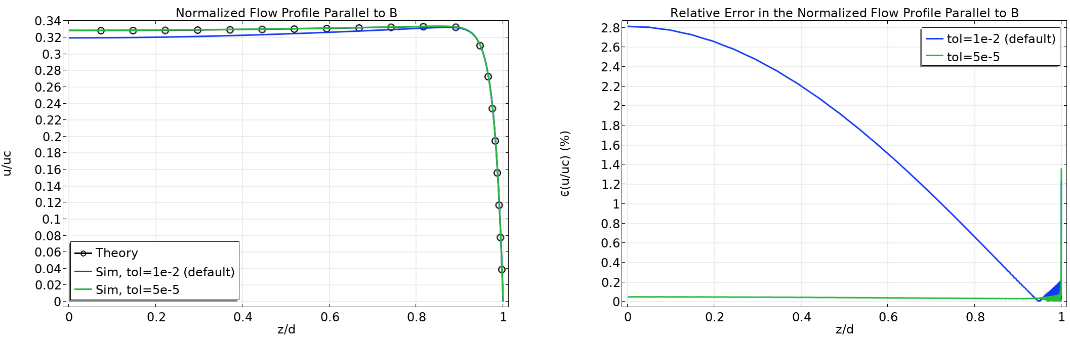Two plots show the normalized flow profile and relative error, respectively. The simulated normalized flow profile parallel to the background magnetic field in Hunt's case for square duct flow when the default tolerance of 1e-2 and a reduced tolerance of 5e-5 are used (left). The asymptotic analytic solution is also plotted for comparison and used to calculate the relative error (right).

As the relative tolerance is reduced, more steps of the nonlinear solver that runs the Newton–Raphson method will be required to solve the model. The number of steps this solver is allowed to take is capped in order to ensure that all models terminate — even ones where no solution can be found that would otherwise run indefinitely. The default cap on the number of steps that can be taken is 200, which is generally suitable for models that are sufficiently load-ramped and use the default tolerance.

However, when too few load ramp steps are taken, or the tolerance is decreased, it is possible for the solver to make good progress toward convergence but fail to meet the tolerance requirement in 200 iterations.

As an example, if the model of Hunt's case for square duct flow is run using a load ramp over the Hartmann number of = 30, 60, and 100; a relative tolerance of 5e-3; and the default maximum number of iterations of 200, the following convergence plot is generated:

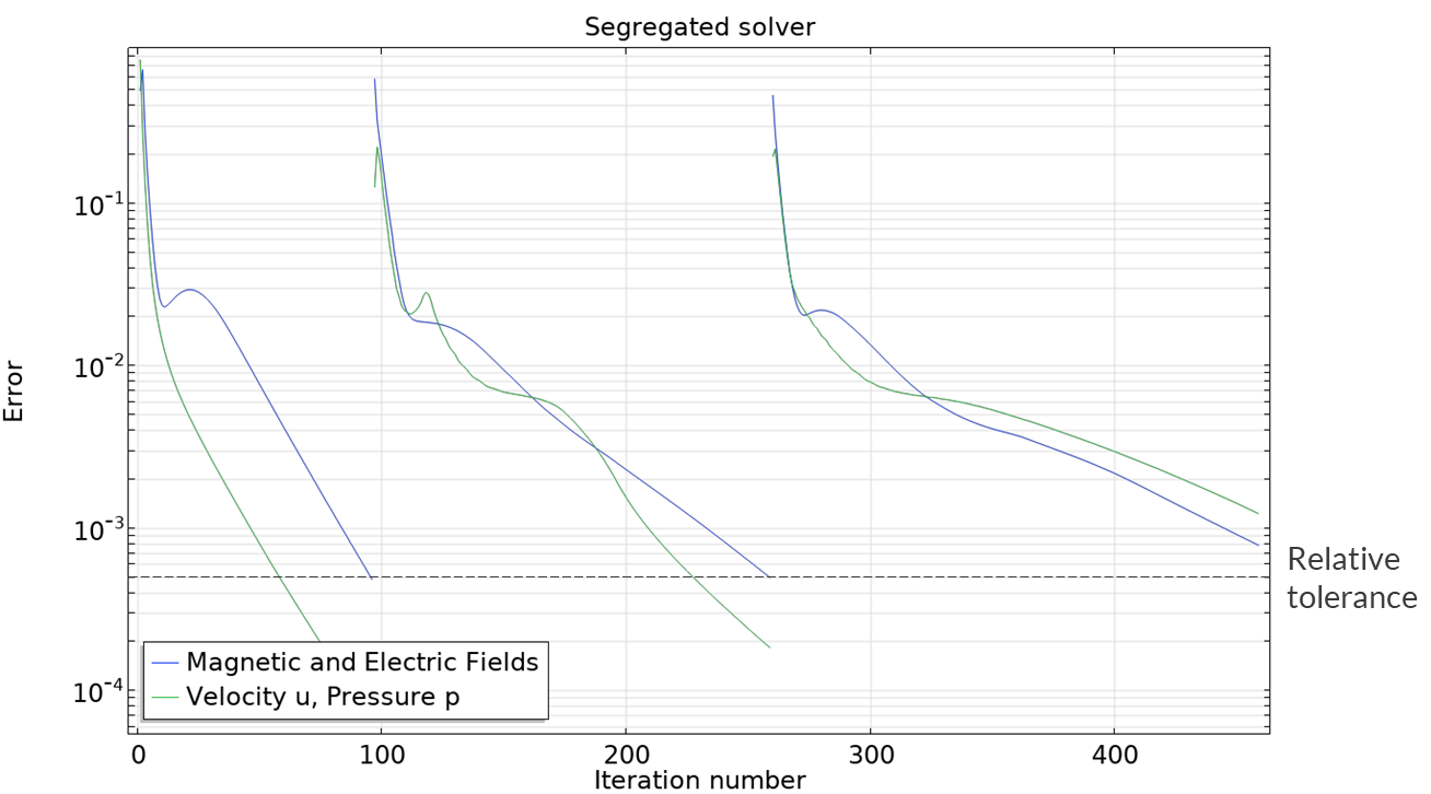
Convergence plot for the example system, with the relative tolerance annotated. The error for each value of that was calculated is displayed on the same plot, with the x-axis showing the total number of iterations taken across the entire simulation.

When the system was calculated for = 30 and 60, the error in both the electromagnetic and fluid flow calculations was reduced below the relative tolerance in under 200 iterations. The solver then increased the Hartmann number and started calculating the next iteration of the system. However, when the Hartmann number was 100, after 200 iterations, the error in the system remained above the relative tolerance. The solver is then terminated and an error message indicates a lack of convergence was the cause. However, considering the convergence plot shows that the error in the system is decreasing smoothly, it can be predicted that convergence would likely be achieved if the solver were allowed to take more iterations.

In this case, the maximum number of iterations that the solver can take can be increased. This is handled in the Segregated solver settings.

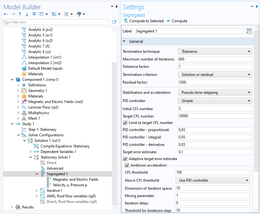The Segregated solver Settings window with an increased number of maximum iterations. Increasing the maximum number of iterations allowed from the default 200 to 600.

If the example system is run again using this higher maximum number of iterations, then convergence is indeed achieved within the iteration limit for = 100.

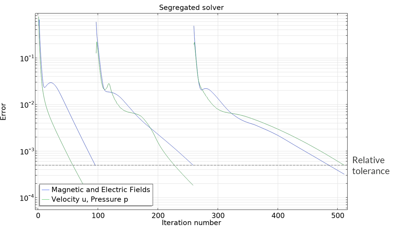
The new convergence plot, showing that convergence is achieved when = 100.

For this test system, the convergence issues when = 100 could also have been resolved by adding additional values into the load ramp over between 60 and 100, e.g., calculating the system for = 80. This would have improved the initial value for the solver when considering the = 100 case, so that it converged within the default 200 iterations. However, computing additional values in the load ramp will also increase the total number of steps taken by the solver.

This gives two methods of improving convergence, both of which will increase the total number of iterations used by the solver but generally by different amounts. Some choice has to be made about which is more computationally efficient in every model. Adding additional load ramp steps has the advantage that the behavior of the system can be studied at more Hartmann numbers, which can be advantageous if this is what the simulation is considering. However, it also generates more data, causing larger file sizes. Allowing additional iterations can be more computationally efficient if the solver is very close to converging within 200 iterations, and solving an additional Hartmann number value would use more iterations than have to be added to the maximum to allow the solver to converge. This must be assessed on a per-model basis.