Modeling with PDEs: Coordinate Transformations
Here in Part 4 of this course on modeling with PDEs using the COMSOL Multiphysics® software, you will learn how to set up an axially symmetric convection–diffusion–reaction PDE by using cylindrical coordinates. One easy method of doing this is to use the built-in physics interfaces for mass transport, as you would simply choose the 2D Axisymmetric option when adding the model component. For educational purposes, this article will focus on how to perform the necessary coordinate transformations by hand and will show you how to implement the axially symmetric equation using the Coefficient Form PDE and General Form PDE interfaces. The techniques used here are applicable to any equation or equation system formulated in cylindrical coordinates and, similarly, spherical coordinates, and can be used when there is no built-in axisymmetric option for your equation or equation systems.
A Tubular Reactor
To illustrate the use of cylindrical coordinates, we are going to set up a simplified version of the Tubular Reactor with Nonisothermal Cooling Jacket tutorial model, first using the Coefficient Form PDE interface and then the General Form PDE interface. The complete model description and model file corresponding to the original model are available through the Application Libraries and the Application Gallery. There, you will also find an app based on the same model.
The tubular reactor model includes a study of the elementary chemical reaction

in a tubular reactor with a liquid phase in the laminar flow regime. In the original model, the reactor is equipped with a cooling jacket to limit the temperature increase (due to the exothermic nature of the reaction) and avoid an explosion. The model is described by the material balances for the species involved and by the energy balances for the reactor and the cooling jacket, as shown in the figure below.
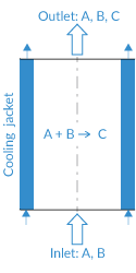
A schematic of the tubular reactor.
In this article, we will use a simplified version of this model; we will ignore the cooling jacket and only model the mass transport and reactions in the reactor under isothermal conditions.
The figure below shows the geometry (a cylinder) of the tubular reactor in 3D.
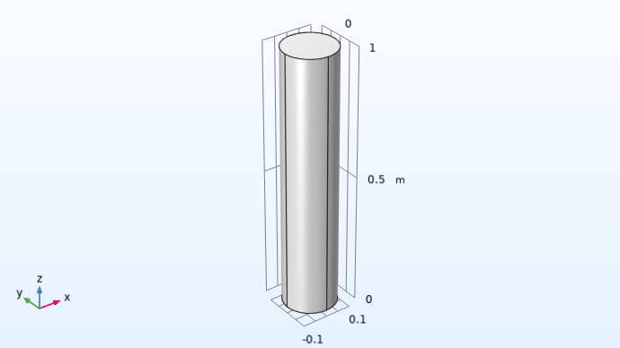
The tubular reactor geometry in 3D.
We will utilize the fact that the boundary conditions and flow pattern exhibit axial symmetry and set up and solve this model in 2D, using a geometry as shown in the figure below.
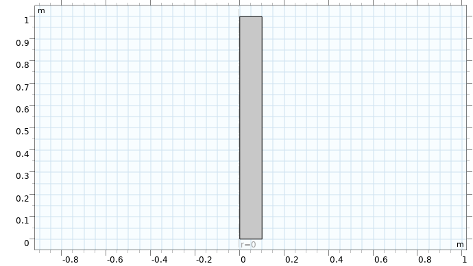
The tubular reactor geometry in 2D as an axisymmetric model.
In the 2D model, what would normally be the y-axis is taken as the axis of symmetry and is renamed the z-axis. In a similar way, the x-axis is renamed the r-axis. For a complete description of the cylindrical coordinates, in addition to the r- and z-coordinates, we also need the azimuthal angle  . However, the assumptions in the model will make it possible for us to later on eliminate the azimuthal angle components.
The reactor will be studied in its steady state so the convection–diffusion–reaction equation, expressed in Cartesian coordinates, that we would like to solve is:

where  is the diffusion coefficient,
  is the concentration of species
  ,
,  is the fluid velocity, and
  is the reaction rate.
Cylindrical Coordinates
In COMSOL Multiphysics®, the Mathematics interfaces always assume that the nabla (or del) symbol  is defined in Cartesian coordinates.
To define the PDE in cylindrical coordinates, we need to first manually perform the necessary coordinate transformation and then match coefficients with the Coefficient Form PDE or General Form PDE, which are always expressed in Cartesian coordinates. More information on cylindrical coordinates is available through other resources.
In cylindrical r-,  -, and z-coordinates, the gradient operator for a scalar field
  is:
is:

and the divergence operator for a vector field  is:
is:

Applying this to our convection–diffusion–reaction equation, we get:

Here, we assume that we have expressed the fluid velocity in cylindrical coordinates so that:

We will now assume that the solution is axially symmetric, which means that all derivatives with respect to vanish. In addition, we can assume that is a constant and then get:

Multiplying this out, we get:

In order to simplify further we need to expand the first term using the chain rule:

We will assume that there is no radial component to the flow so that:

Putting all this together, we get:

We can rearrange this a bit to get:

This formulation is almost ready to use for coefficient matching. However, we have an issue with division by zero if  , which happens on the axis of symmetry.
To get around this, we can simply multiply the equation by  to get:

This issue with division by zero is bound to happen when transforming the equations into cylindrical, or spherical, coordinates. As opposed to the Mathematics interfaces, the built-in physics interfaces for 2D axisymmetry handle this automatically.
To match this PDE with the Coefficient Form PDE template, we need to first "forget" that we are working with cylindrical coordinates and identify:

and then compare it with:

We see that we can put:


Note that the convection coefficient  does not include the x-component
  . The reason for this is that it is already implicitly included due to the fact that the diffusion coefficient depends on . When we identified , we implicitly pulled this coefficient inside of the divergence operator. To see how this works, we need to be careful with applying the chain rule "backward". When we apply the divergence operator on the diffusion term:

with  we get, from the chain rule, an extra term in the r direction. To see this, write each component separately:

The partial derivatives with respect to gives:

and the first term in this expression is already present in the equation derived earlier.
This shows that in order to implement PDEs in cylindrical, or also spherical, coordinates, it is necessary to derive the transformed equations carefully since there may be nonintuitive contributions to the coefficients in the Coefficient Form PDE or the General Form PDE.
The Tubular Reactor Parameters
In the tubular reactor model, the diffusion coefficient is taken to be a constant  m2/s.
m2/s.
The velocity is assumed to have a known parabolic profile:

where  is the average velocity,
  is the tubular reactor radius, and is the radial coordinate.
The reaction rate is the Arrhenius expression:

where  is the activation energy, is the frequency factor,
  is the gas constant, and
  is a constant temperature, since we assume the reactor to be isothermal. In reality, the reactor is, of course, not isothermal. This more realistic modeling scenario is covered in the tubular reactor tutorial model, where
  is the dependent variable of a heat transfer equation that is solved simultaneously with this convection–diffusion–reaction equation.
Boundary Conditions
Now that we have identified the coefficients and the dependent variable of the equation
as

we know that the Neumann boundary condition:

takes the form

where the coefficients  and
and  can be chosen to model a variety of phenomena on the boundary.
The Dirichlet condition is:

and is not affected by the coordinate transformation. In the tubular reactor example, we will have this Dirichlet boundary condition at the inlet.
We would like the chemical species to be transported through the outlet without hindrance. We can achieve this by using the Neumann boundary condition:

In this way, we are not getting any artificial contribution to the mass transport through the boundary from the diffusive flux term, but all mass transport will implicitly come from the convective equation term:

Using the Coefficient Form PDE for the Tubular Reactor
To set up the tubular reactor model using the Coefficient Form PDE interface, start a new model using the Model Wizard and in the Select Space Dimension window select the 2D Axisymmetric option, as shown in the figure below.
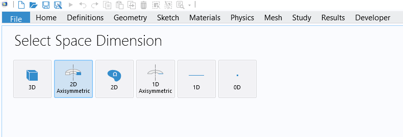
The 2D Axisymmetric option for the spatial dimension of the model component.
On the next Select Physics page, select the Mathematics interface Coefficient Form PDE, change the Field name and Dependent variables fields to cA, and change the units to Concentration and Reaction rate, respectively. You do this using the Physical Quantity dialog box, where the Concentration unit is located under General and the Reaction rate is located in the Transport folder, as shown in the figure below.
The settings for the Coefficient Form PDE interface.
Following this, on the next Select Study page, select a Stationary study.
The geometry model is a simple rectangle with width 0.1 and height 1.0, as shown in the figure below.
The model geometry.
When we originally selected the 2D Axisymmetric option in the Select Space Dimension page of the Model Wizard, we get an automatic renaming of the x- and y-coordinates into r and z, respectively. In addition, we get a dashed line representing the axis of symmetry along the z-axis at r = 0. For the geometry, it is required that all parts have a radial coordinate greater than or equal to zero. You should think of the geometry as being revolved 360 degrees around the symmetry axis.
For the built-in physics interfaces, the governing equations are automatically transformed (through multiplication by , etc.) when you select the 2D Axisymmetric option for spatial dimension of the model component. However, for the Coefficient Form PDE and General Form PDE, no transformation of the equations are made. Instead, you have to perform these transformations manually, as described above.
Before defining the PDE coefficients, we need to define a number of parameters and variables. These parameters are taken from the tubular reactor tutorial model, where you can find more information on the chemical engineering aspects of this simulation. You can load the parameters and variables (shown below) into the model by downloading the text files that are associated with this article.
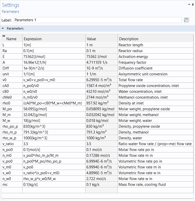
The global parameters for the tubular reactor model.
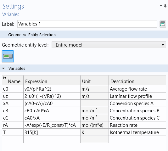
The variables for the tubular reactor model.
The isothermal temperature is defined here as a variable with the value 315 K. If you wanted, you could extend the model with another equation for heat transfer and then remove this variable.
There are a few discrepancies in notation between the model and the derivation. For example, the parameter for the diffusion coefficient is named Diff in the model and the species concentration is named cA.
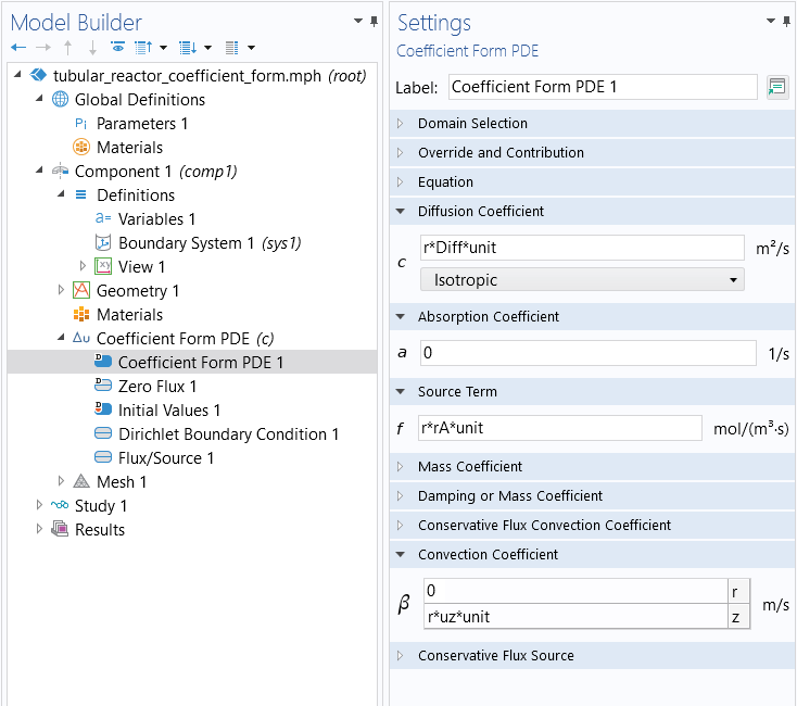
The Coefficient Form PDE node settings are shown in the figure below. Notice that we have introduced a unit scaling parameter, unit, in order to compensate for the fact that we have multiplied the entire equation by to avoid division by zero on the symmetry axis. This parameter has the value 1[1/m] to eliminate the length unit coming from multiplying it by . Alternatively, we could have used other units in the Model Wizard. However, in that case we would have needed to modify the units of all the parameters, so introducing this scaling factor is more convenient.
The Coefficient Form PDE node settings for the tubular reactor model.
The lower boundary has a Dirichlet Boundary Condition for the fixed concentration at the inlet, as shown in the figure below.
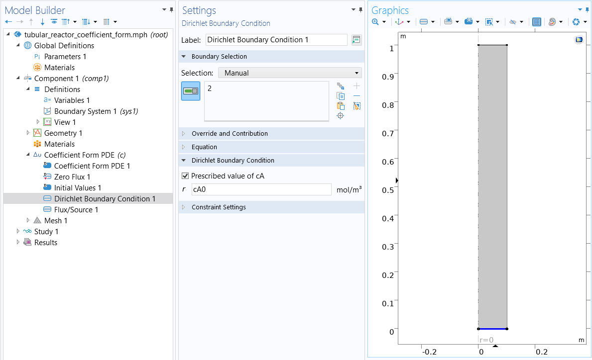 The COMSOL Multiphysics UI showing the Model Builder with Dirichlet Boundary Condition selected, the corresponding Settings window, and the Graphics window showing the tubular reactor model geometry.
The Dirichlet Boundary Condition at the inlet.
The COMSOL Multiphysics UI showing the Model Builder with Dirichlet Boundary Condition selected, the corresponding Settings window, and the Graphics window showing the tubular reactor model geometry.
The Dirichlet Boundary Condition at the inlet.
The upper boundary has the outflow condition , as shown in the figure below.
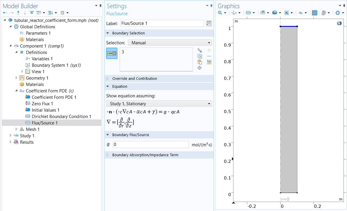 The COMSOL Multiphysics UI showing the Flux/Source selected in the Model Builder, the corresponding Settings window, and the Graphics window.
The outflow Neumann boundary condition.
The COMSOL Multiphysics UI showing the Flux/Source selected in the Model Builder, the corresponding Settings window, and the Graphics window.
The outflow Neumann boundary condition.
For this model, we use the same mapped mesh settings as in the original tutorial model, as shown in the figure below.
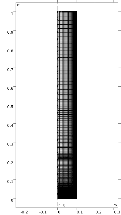
The mapped mesh used in the tubular reactor model.
After solving, we get a plot of the concentration throughout the reactor, as shown in the figure below.
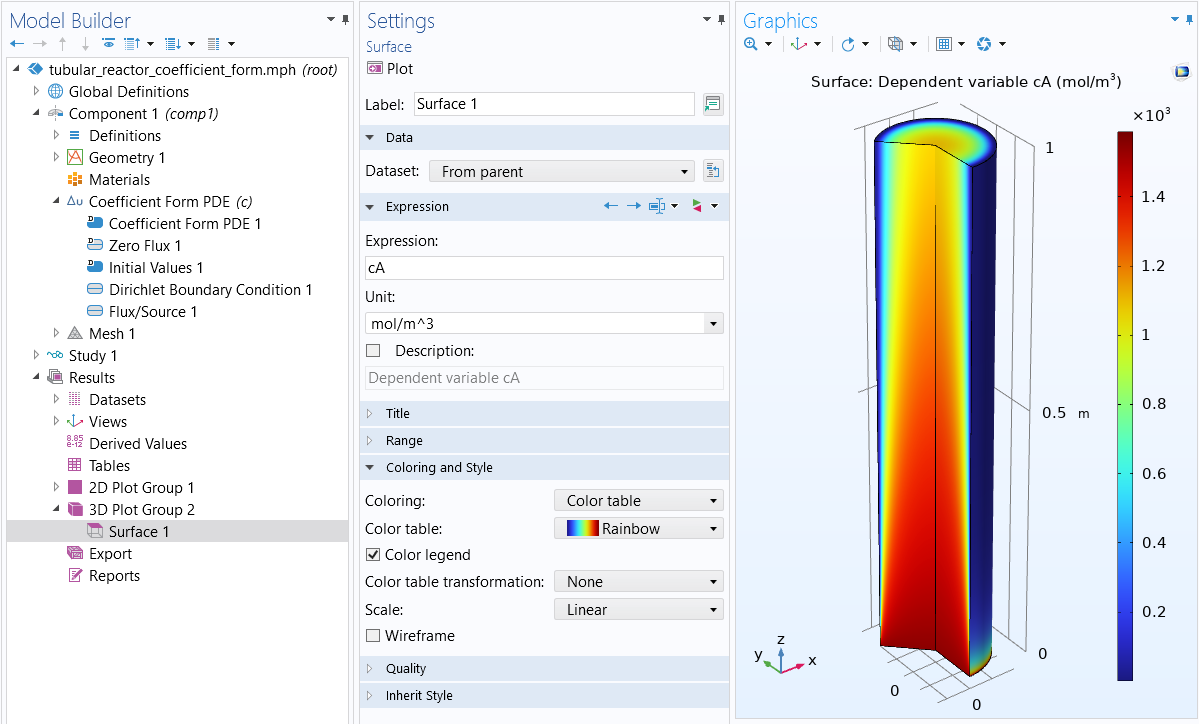
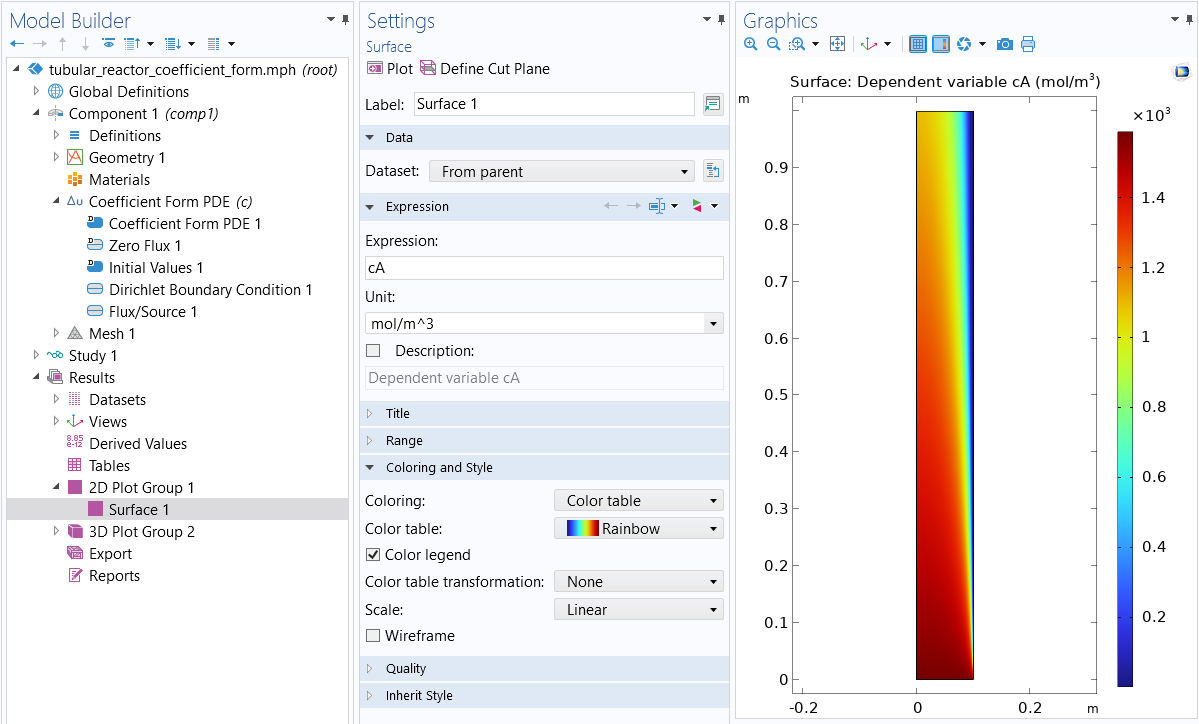 The COMSOL Multiphysics UI showing the Model Builder with Surface 1 selected, the Surface Settings window, and the Graphics window with the 2D model shown in the Rainbow color table.
The concentration
of species in the reactor.
When using the 2D Axisymmetric option, we automatically get a revolved dataset plot with a cutout, as shown in the figure below.
 The Model Builder with Surface 1 selected, the corresponding Settings window, and the Graphics window with the model in 3D.
A 3D visualization of the concentration of species .
The Model Builder with Surface 1 selected, the corresponding Settings window, and the Graphics window with the model in 3D.
A 3D visualization of the concentration of species .
This is one of the additional benefits we get from using the 2D Axisymmetric option when setting up the model.
Since the list of Variables also included expressions for the species  and
and  we can plot them as well. The figure below shows a plot of the concentration
  of species .
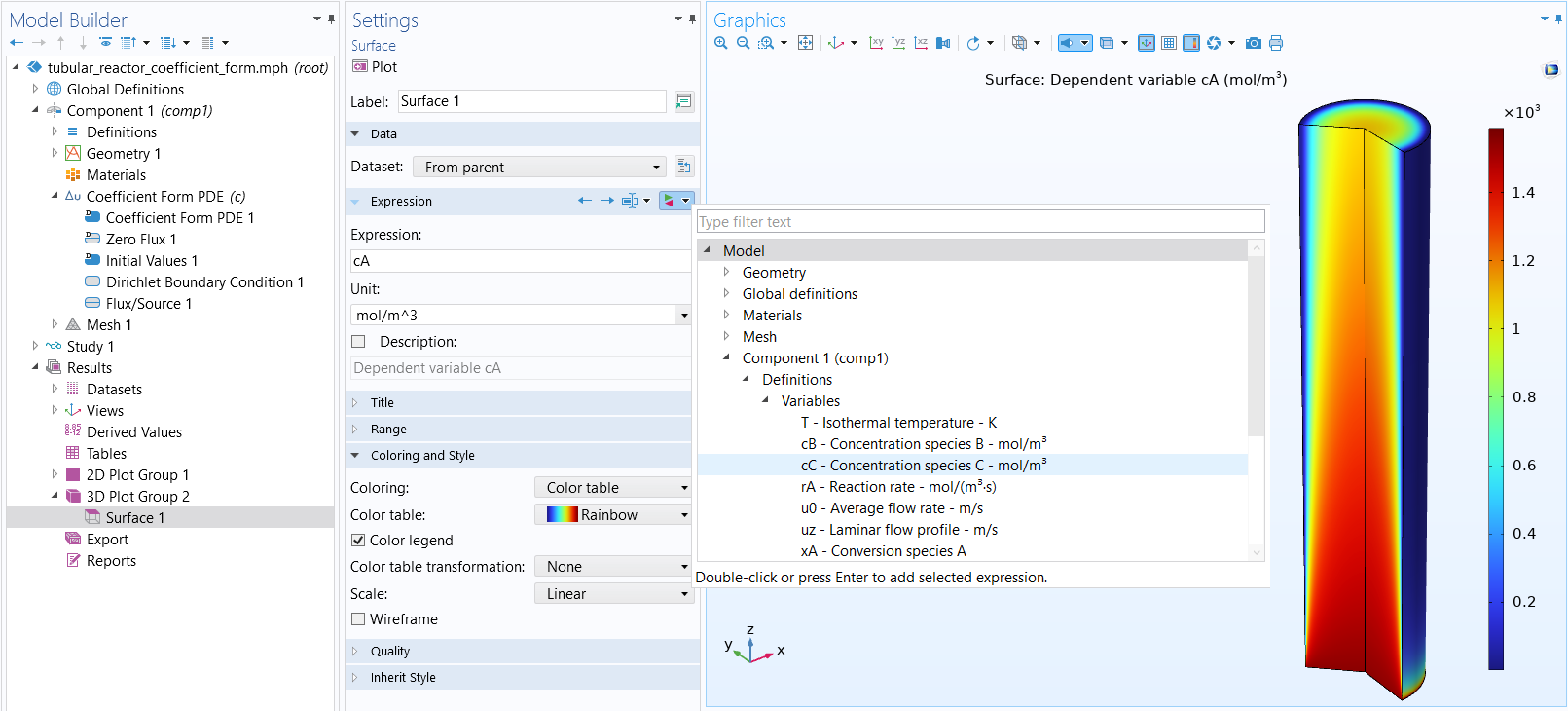 The Model Builder with Surface 1 selected, the corresponding Settings window with Concentration species C selected, and the Graphics window with a 3D version of the model.
A 3D visualization of the concentration of species .
The Model Builder with Surface 1 selected, the corresponding Settings window with Concentration species C selected, and the Graphics window with a 3D version of the model.
A 3D visualization of the concentration of species .
The list of files that you can download from this article includes a version of the tubular reactor using the Coefficient Form PDE interface as well as a version using the Transport of Diluted Species interface so that you can compare the two. The results are more or less identical.
Note that since this model includes convection we might wonder if we need some numerical stabilization to avoid oscillations. This is not needed since the model has a fair amount of diffusion compared to convection and since the mesh is quite fine (which reduces the need for numerical stabilization).
Using the General Form PDE for the Tubular Reactor
Using the General Form PDE interface is very similar to that of the Coefficient Form PDE interface. Recall that the relationship between the stationary Coefficient Form PDE and General Form PDE is:


with

and

This means that for the tubular reactor we get:


Note that in the software, the gradient components

are called cAr and cAz, respectively. The derivative components of a dependent variable, up to degree 2, are always available in the software for use in expressions as the name of the dependent variable with the spatial components appended. In the case of x-, y-, and z-coordinates, if the dependent variable is u, then the derivative components are ux, uy, uz, uxx, uxy, and so on. In this case, the dependent variable is cA, the coordinate variables are r and z, so the derivatives are cAr, cAz, cArz, and so on.
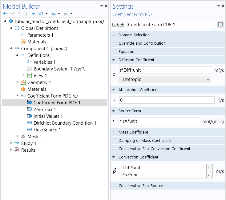
For the General Form PDE, this means that the components of the Conservative Flux  are entered as:
-r*Diff*cAr*unit
-r*Diff*cAz*unit
where, just like in the Coefficient Form PDE interface version, the unit parameter is used to compensate for the fact that we have multiplied the equation with .
The Source Term is entered as:
(r*rA+Diff*cAr-r*uz*cAz)*unit
This is the only difference compared to the version based on the Coefficient Form PDE. The corresponding settings for the General Form PDE is shown in the figure below.
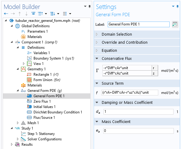
The General Form PDE node settings for the tubular reactor model.
The list of files that you can download from this article also includes a General Form PDE version of the tubular reactor with identical results to that of the version based on the Coefficient Form PDE.
Built-In Axisymmetric Interfaces
In the Model Wizard, there are several built-in interfaces that can be used for quickly setting up models similar to the tubular reactor example. The most important ones are the Transport of Diluted Species interface, available under the branch for Chemical Species Transport, and the Stabilized Convection-Diffusion Equation, available under Mathematics Interfaces>Classical PDEs. These built-in interfaces take care of the multiplication by and there is no need to perform the coordinate transformations by hand.
Submit feedback about this page or contact support here.