Modeling with PDEs: Diffusion-Type Equations
Here in Part 2 of this course on modeling with partial differential equations (PDEs), we will have a closer look at using the Coefficient Form PDE and General Form PDE interfaces to model with general diffusion-type equations, such as Poisson's equation, the Laplace equation, and the heat equation. For conventional modeling and simulation tasks, there is no need to use a mathematics interface. Instead, you can simply use a built-in physics interface. However, if you want low-level control over all aspects of your equation-based models, using a mathematics interface is a great option.
The PDE Interfaces
The PDE interfaces in COMSOL Multiphysics® can be used for specifying linear and nonlinear partial differential equations, including many of the classical PDEs:
- Laplace equation
- Poisson's equation
- Convection–diffusion equation
- Wave equation
- Helmholtz equation
- Heat equation
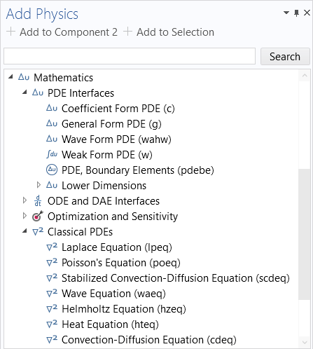
These PDEs are ubiquitous in physics and can all be cast into a generic form containing derivatives up to the second order in both time and space. Below, in the Select Physics window of the Model Wizard, you can see the options that are available for PDE modeling. The classical PDEs listed earlier are available under the Classical PDEs branch.
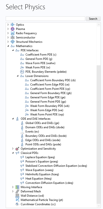
The interface options for PDE modeling in the Model Wizard.
In the list of PDE Interfaces, you will find the Wave Form PDE, which is an interface for conducting numerical experiments and modeling based on the discontinuous Galerkin method. We will not be discussing the Wave Form PDE or Classical PDEs interfaces in this course, but instead cover how to use the general-purpose interfaces for PDE modeling. This includes the Weak Form PDE interfaces and the interfaces found under Lower Dimensions and ODE and DAE Interfaces in the Model Wizard.
The Coefficient Form PDE
One of the most valuable equation-based modeling tools in COMSOL Multiphysics® is the Coefficient Form PDE. (We will go into detail on how to use this interface here as well as in other parts of this course.) Later in this article, we will also learn about the General Form PDE interface. These two equation forms, or equation templates, are more or less equivalent in terms of the equations they can express. They also provide modeling capabilities for specifying coefficients for the derivatives of different orders up to order two. PDEs of an order higher than two can be modeled using a system of PDEs, as shown here.
Let us first recall some notation from vector calculus for the gradient and divergence of a scalar field,  , and vector field,
  :
:


The Coefficient Form PDE for one dependent variable, , with isotropic coefficients is written as follows:

There are two important boundary conditions when using this interface. First, is the generalized Neumann boundary condition:
 ,
,
which is used for modeling a boundary flux. The second is the Dirichlet boundary condition:

which is used for assigning fixed values to the dependent variable on the boundary.
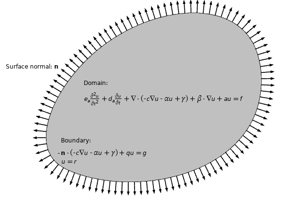
The PDE with boundary conditions for a Coefficient Form PDE.
If there is one dependent variable in the Coefficient Form PDE and all of the materials are isotropic, then most of the coefficients will be scalar quantities, except for the following, which are always vector-valued:
Scalars: 
Vectors: 
Note that when modeling anisotropic materials, some of the scalar coefficients instead become vectors or matrices (tensors).
In the examples farther below, we will see how we can use the Coefficient Form PDE to define some of the classical PDEs by matching their coefficients.
What about defining spatially varying coefficients or nonlinear equations? In COMSOL Multiphysics®, the equation coefficients can be defined as expressions in terms of:
- The spatial coordinates x, y, and z
- The time variable, t
- Complex-valued expressions such as
1+j*sqrt(5) - The dependent variables (u, v, w,...)
- The derivatives of the dependent variables:
ux,uy,uz,uxx,uxy, and so on - User-defined functions and lookup tables
This is also true when using built-in physics interfaces, i.e., material properties, sources, loads, etc., can also be defined as expressions.
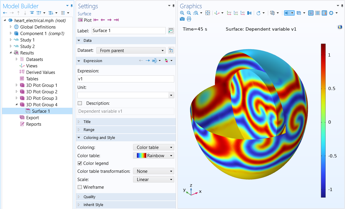 The COMSOL Multiphysics UI with Surface 1 selected in the Model Builder, the corresponding Settings window, and a model of electrical activity in cardiac tissue in the Graphics window.
Modeling the electrical activity in cardiac tissue using the General Form PDE mathematics interface. In this model, two different time-dependent nonlinear partial differential equation systems are used: the FitzHugh–Nagumo equations and the Ginzburg–Landau equations. This model was kindly provided by Prof. Simonetta Filippi and Dr. Christian Cherubini from University Campus Biomedico di Roma, Italy.
Naming of the PDE Coefficients
The names of the different terms in the Coefficient Form PDE interface are inspired by transport equations.
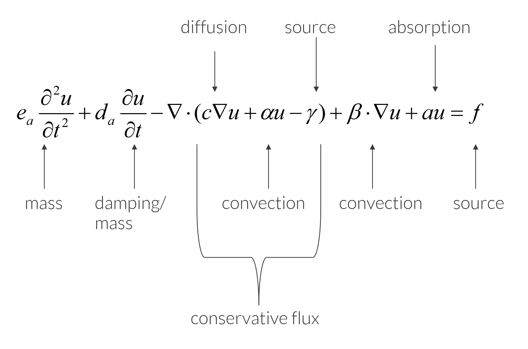
The terminology convention for the various terms in the Coefficient Form PDE.
In this article, we will go through some of the different PDE terms and the background of their names.
Poisson's Equation
The Coefficient Form PDE may look complicated, especially if you have not seen it before. To break this down a bit, let us first consider the stationary version of this equation, where we assume that all transient phenomena have ceased. In other words, we assume that:

for all times of interest. This also means that we ignore the influence of the coefficients  and
and 
The stationary version of the Coefficient Form PDE reads:

To simplify this even further, let us assume that:


We now end up with the equation (moving the negative sign in front):

which is a generalized form of Poisson's equation. The sign convention is chosen so that  corresponds to a source and
  corresponds to a sink.
If we set  , then we get the classical Poisson's equation.

If we set  , we get the Laplace equation.
Sometimes it is more convenient to model a source using the conservative source term,  . For some examples of this, you can review the table of commonly used equations at the end of this article.
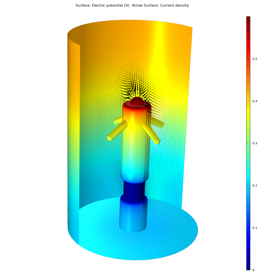 The Laplace equation is one of the most common PDEs for real-world applications. In this case, the Laplace equation is used for modeling the conservation of currents in biological tissue surrounding a pacemaker electrode. The visualization shows the electric potential (color) and current density (arrows).
The process of identifying coefficients in the Coefficient Form PDE, as demonstrated earlier, is representative of how you can use this equation template for real modeling tasks:
- Start by considering if the equation is stationary or time dependent.
- Eliminate the time-dependent terms if needed.
- Further eliminate unnecessary coefficients.
- Match the coefficients of your equation with those remaining in the Coefficient Form PDE.
The figures below show the default settings for the scalar version of the Coefficient Form PDE when a stationary study is selected. The default coefficients correspond to Poisson's equation.
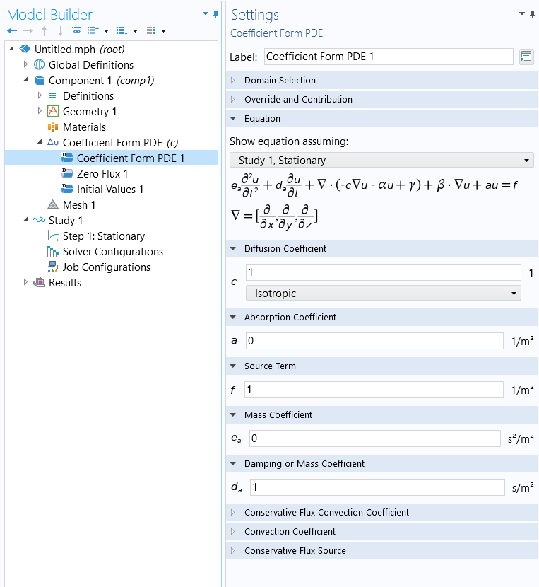
The default scalar coefficients for the Coefficient Form PDE node, corresponding to Poisson's equation.
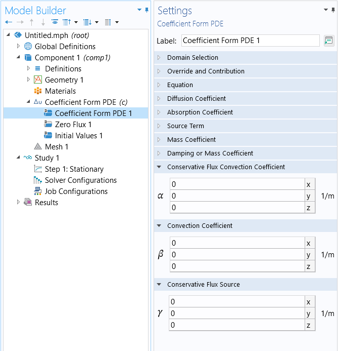
The vector-valued coefficients in the Coefficient Form PDE node.
You may notice that the coefficient of the first-order time derivative is, by default,  . This coefficient is only active if we have selected a Time-Dependent or an Eigenvalue study type. For more information on eigenvalue equations, see Part 7. For a stationary study, this coefficient does not have influence since for a stationary PDE .
To see an example of using the Coefficient Form PDE for modeling Poisson's equation, read Part 1 of this course, which focuses on solving the Laplace and Poisson's equations for the gravitational field of the Earth–Moon system.
The Heat Equation
Let us now see how we can match the coefficients of the Coefficient Form PDE with those of the time-dependent heat equation:

where  is the temperature,
  is the density,
  is the heat capacity,
  is the thermal conductivity, and
  is a volumetric source term. The source term can, for example, be the heat generated by a chemical reaction or an electric current.
If we compare this with the Coefficient Form PDE:
we see that


In the Model Wizard, as an alternative to using the Coefficient Form PDE, there is a dedicated Heat Equation interface, which is grouped together with interfaces for a number of other common PDEs. These are available as predefined mathematics interfaces under Classical PDEs, as shown in the figure below. For full-fledged heat transfer modeling, you can instead use the Heat Transfer in Solids interface or any of the built-in physics interfaces available under the Heat Transfer branch.
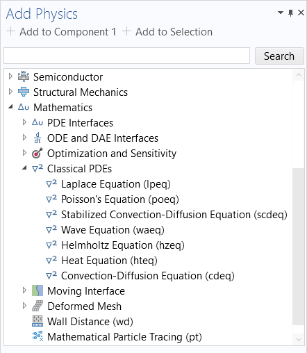
The interfaces for classical PDEs, available through the Add Physics window or in the Model Wizard.
Note that in the heat equation, if we set  we get the stationary heat equation, which is the same as the generalized form of Poisson's equation:

To change the name of the dependent variable from to , go to the Coefficient Form PDE node and change the settings in the Dependent Variables section, as shown below.
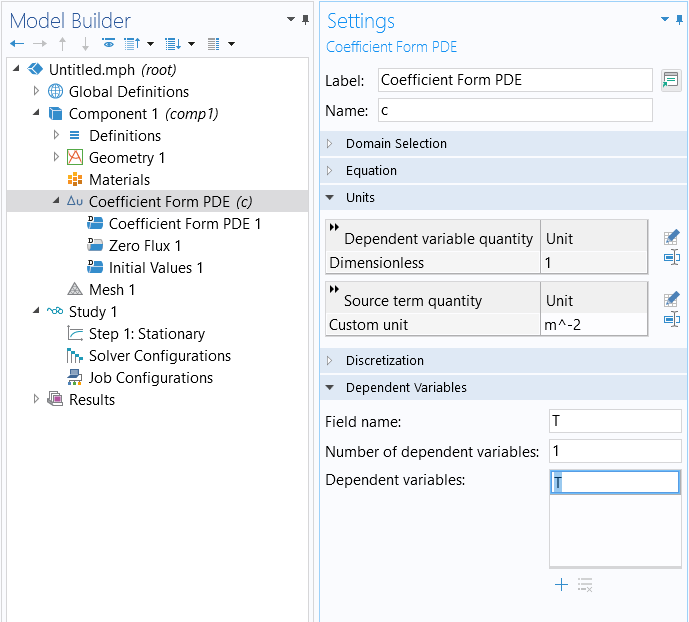
Changing the name of the dependent variable for the Coefficient Form PDE.
The Field name is the name of the physical field, which in general can be vector-valued. The individual scalar field component variables are defined under Dependent variables. For the heat equation, we can define the Field name and Dependent variable name to be the same.
Understanding Boundary Conditions and Flux
The Dirichlet condition:
is used for setting a value to the dependent variable on a boundary. Depending on which physics that the PDE is describing, this value can be, for example, a temperature, voltage, or concentration. In cases where the PDE, or system of PDEs, is describing structural mechanics, this boundary condition is used for setting a prescribed displacement on a boundary. In later articles, we will encounter structural mechanics PDEs.
The generalized Neumann boundary condition
represents the flux on the boundary. To understand this boundary condition we need to compare with the stationary Coefficient Form PDE:
We see that the expression within the parentheses is the same for the PDE and the Neumann boundary condition:

This quantity:

represents the domain flux of the PDE. In the case where the PDE represents a conservation law, this part of the PDE typically represents the quantity that is conserved.
For example, if the PDE is the heat equation, the flux is

which is Fourier's law of thermal conduction.
The PDE term

represents the local conservation of heat flux.
In a stationary case without a heat source we get:

which tells us that there is a heat balance for each infinitesimal control volume. In other words, "what goes in must go out". For more information on conservation laws, see here.
The term  describes a diffusion process and, because of this, the heat equation is sometimes viewed as a version of the diffusion equation.
In a time-dependent case without a heat source we get:

which we can write as

where the term

from a conservation point of view can be seen as a source term and represents the local absorption or release of locally stored heat.
If we now go back to the generalized Neumann boundary condition, we can see that for the heat equation this boundary condition reads:

The term  represents the heat flux across the boundary. If we want to provide more heat to the modeling domain, we can use a positive boundary heat flux source
  term . If we want to provide cooling, then
  .
.
The term  can have several different physical meanings. In the case of heat transfer, the simplest interpretation is perhaps that of Newton's law of cooling, which assumes that the cooling on the boundary is directly proportional to the temperature difference according to:

where  is the heat transfer coefficient and
  is a fixed ambient or external temperature. If we now rearrange this equation we get:

and we can match coefficients to see that:


So, in general,  represents a boundary flux and
  represents some kind of film, layer, or membrane conductance.
For comparison, in the case of structural mechanics, can be interpreted as a stiffness density, also known as spring constant density, of an elastic layer. For structural mechanics, the dependent variables and coefficients are vectors and tensors rather than scalars. The Solid Mechanics interface in the Structural Mechanics Module and MEMS Module have built-in functionality for elastic layers and spring constant densities.
The General Form PDE
The General Form PDE interface is a compact alternative to the Coefficient Form PDE interface:

with associated generalized Neumann and Dirichlet boundary conditions:


Here,  is the domain flux expressed in terms of the gradient of the dependent variable .
In the Dirichlet condition,  is an equation in the dependent variable . This equation is set to zero on the boundary where this condition is applied. For example, to set the value on the boundary to 1, you would define as

We can use the General Form PDE to get Poisson's equation by setting:


This is the default setting for the General Form PDE node, as shown below.
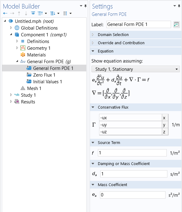
The default settings for the General Form PDE node, corresponding to Poisson's equation.
Note that the time-dependent coefficients are inactive if we use a stationary study.
In general, this equation is just as expressive as the Coefficient Form PDE. We can see this by converting the Coefficient Form PDE to the General Form PDE as follows:

This is possible in the COMSOL Multiphysics® user interface since we are allowed to use derivatives of dependent variables by using syntax according to the following table:
| Mathematical Notation | User Interface Syntax | Alternative User Interface Syntax |
|---|---|---|
 |
ux | d(u,x) |
 |
uy | d(u,y) |
 |
uz | d(u,z) |
When defining Poisson's equation, each of the gradient components are entered in the user interface for the different flux components of  , but with a negative sign.
The General Form PDE can express the exact same equations as the Coefficient Form PDE. Which one you use is only a matter of convenience. As long as you express the same equation or system of equations, there is no difference in terms of convergence, accuracy, etc. between the two equation forms.
Diffusion Equations for Common Industrial Applications
Different versions of the diffusion equation form the basis of several built-in physics interfaces in COMSOL Multiphysics®. The table below summarizes some of the most commonly used versions (click on the table to enlarge it):
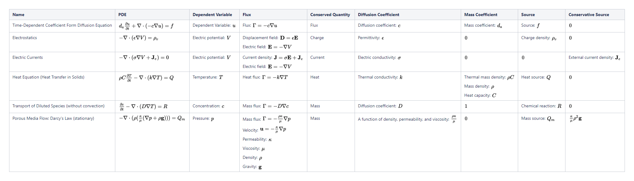 A table showing interfaces that correspond to different kinds of diffusion equations with columns for the PDE, dependent variable, flux, conserved quality, coefficients, and sources.
Further Learning
The figure below shows the Equation Based models that are available in the COMSOL Multiphysics branch of the Application Libraries. The models do not require any add-on products and span many different application areas.
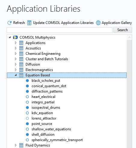
The Equation Based example models in the Application Libraries.
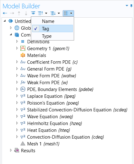
Here, you will find introductory examples of models that use the Mathematics interfaces, including the Coefficient Form PDE interface, General Form PDE interface, and Weak Form PDE interface. The Mathematics interfaces are also used in other models in the Application Libraries. To learn more about how these mathematics interfaces were used in models as well as the logic behind doing so, you can search the appropriate tag in the Application Libraries. For example, if you wanted to see a list of models that use the Coefficient Form PDE interface, you would enter @tag:c or @physics:c in the search field.
Submit feedback about this page or contact support here.