Problem Description
Why do I get negative values of the concentration in my diffusion, convection and reaction model? Why do I see values that go below, or above, their lowest, or highest, possible values based upon the boundary conditions applied for problems involving diffusion and convection? It is clearly unphysical.
Solution
There are several possible reasons for, and ways to avoid the issue of over- and under-shoot of the solution:
Numerical Errors
A common reason is numerical noise: For example, when the variable for concentration approaches zero, the numerical noise may become significant in comparison to the value (which is close to zero). If you notice negative concentrations of very small magnitude, numerical noise is probably the cause and does not affect the problem much in diffusion/convection problems without reactions.
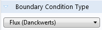
Reacting Domains: Use Danckwerts inflow type
If you have an inlet to a domain with a chemical reaction, or a domain with reactions on the walls, use the Inflow condition, and set Boundary Condition Type: Flux (Danckwerts), available in the Inflow settings. This inflow condition type is designed to avoid negative oscillations and also to speed up the solution of reacting flow problems.
 .
.
For an example how to use this, see Separation Through Dialysis.
Discontinuous Boundary and Initial Conditions: Smoothen the Settings
Another cause for locally slightly negative concentrations is a discontinuity in space or time, for instance in the initial condition. As an example, consider the one dimensional time dependent Convection-Diffusion-Reaction equation:

The initial condition is zero concentration within the domain and the boundary conditions are set to 1 and 0 concentration at the left and right boundary, respectively. The physical interpretation of this is an initially sharp, gradually diffusing front moving in the positive x-direction. However, for finite element shape functions (e.g. first order Lagrange), only continuous functions are admissible as solutions, for which reason the discontinuous initial value is modified before the time-iterations can begin. This often results in a small dip in the solution for t=0. The dip traverses to the first time steps too. The concentration will locally be slightly negative at t=0, as shown in the figure.
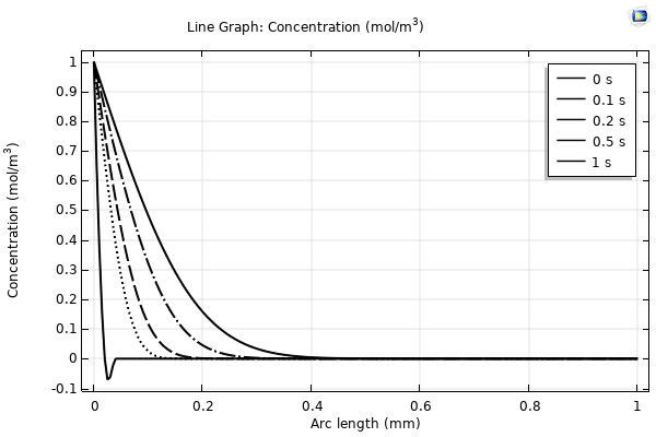
Figure 1: Solutions to the time-dependent diffusion problem with a boundary condition at the left (c=1) that creates a discontinuity with the initial condition (c=0) at t=0. The finite element method gives rise to a swing below zero in the leftmost element. The dip close to t=0 sometimes results in oscillations and convergence problems.
This problem can be avoided by using one of COMSOL Multiphysics's built in smoothed step functions smooths out the initial discontinuity in a controlled way. For instance, in the example above, you could, instead of the uniform zero initial condition, use a smoothed step transition as the initial condition. For more information please refer to Solution 905: Modeling of step transitions.
Condition the Reaction Term to be Larger than Zero for Concentrations Approaching Zero
A significant negative concentration often indicates that the underlying mathematical model does not correctly describe the physics. In this case the approach mentioned above does not take care of the problem. One potential cause is that you have a constant sink in your reaction term, which is an approximation that only works for large concentrations. When the concentration reaches zero, the reaction term continues to consume the species, finally resulting in negative concentration. This can be avoided by making sure that your reaction rate is such that when the concentration of the species approaches zero, then so does the species sink. This can be achieved for instance by writing max(eps^2,Q). eps is an internal COMSOL constant that is a very small number in the order or 10-15. This type of expression is also helpful if you want to avoid Q being 0, for example if you apply the logarithm to it somewhere within the geometry, or if the symbolic derivative runs a risk of containing division by zero.
Make Sure the Mesh Resolves the Problem
Insufficient mesh resolution can result in dips below zero. Convergence problems are often the underlying issue when negative concentrations are observed in high convection regimes (high Péclet number) and with large reaction terms or fast kinetics (high Damköhler number). It can also be useful to investigate whether the negative concentration gets better or worse with mesh refinement. If better, the problem is most likely mesh related. If worse, it is probably the mathematical model that causes the problem.
Solving a convection-dominated convection-diffusion equation with equation-based modeling.
If you are solving a convection-dominated equation with either the Coefficient Form PDE, General Form PDE, or Weak Form PDE, oscillations may occur because none of these interfaces include any numerical stabilization. You may be able to use the Stabilized Convection-Diffusion Equation instead - it contains streamline diffusion and crosswind diffusion stabilization, active by default. The Stabilized Convection-Diffusion Equation is available in 3D, 2D Axisymmetry, 2D, and 1D, and can be found under the Mathematics>Classical PDEs branch when adding a physics interface.
In Knowledge Base solution 103: Improving Convergence of Nonlinear Stationary Models a few other approaches are presented which may alleviate these types of problems without extensively refining the mesh.
Related Files
| conc.mph | 445 KB |
| Model that creates the plot above. | |
COMSOL makes every reasonable effort to verify the information you view on this page. Resources and documents are provided for your information only, and COMSOL makes no explicit or implied claims to their validity. COMSOL does not assume any legal liability for the accuracy of the data disclosed. Any trademarks referenced in this document are the property of their respective owners. Consult your product manuals for complete trademark details.