Postprocessing and Visualization Updates
COMSOL Multiphysics® version 6.0 brings a new feature to cap faces when using interactive clipping, arrays of plots, and new color tables. Browse all of the postprocessing and visualization updates below.
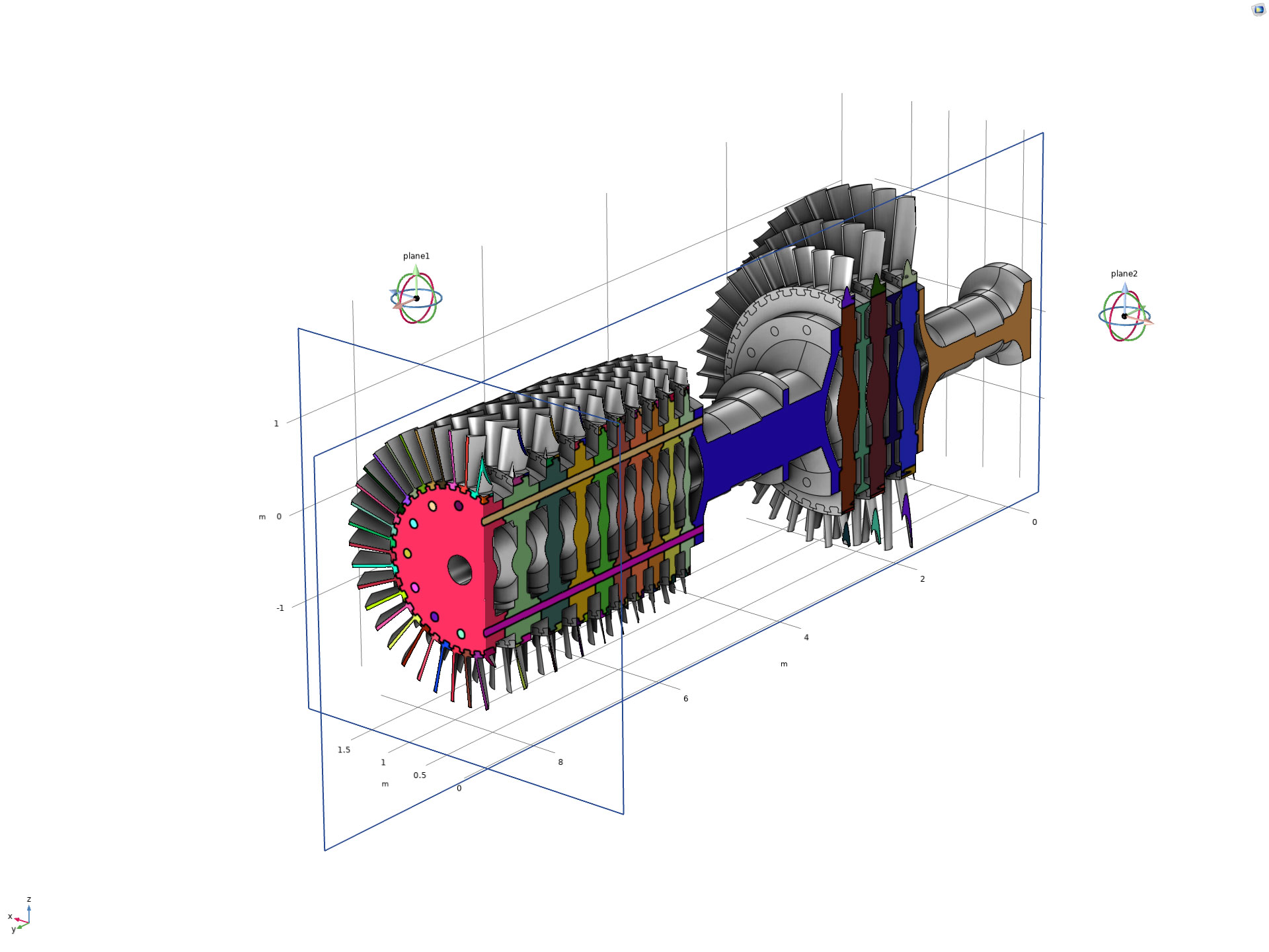
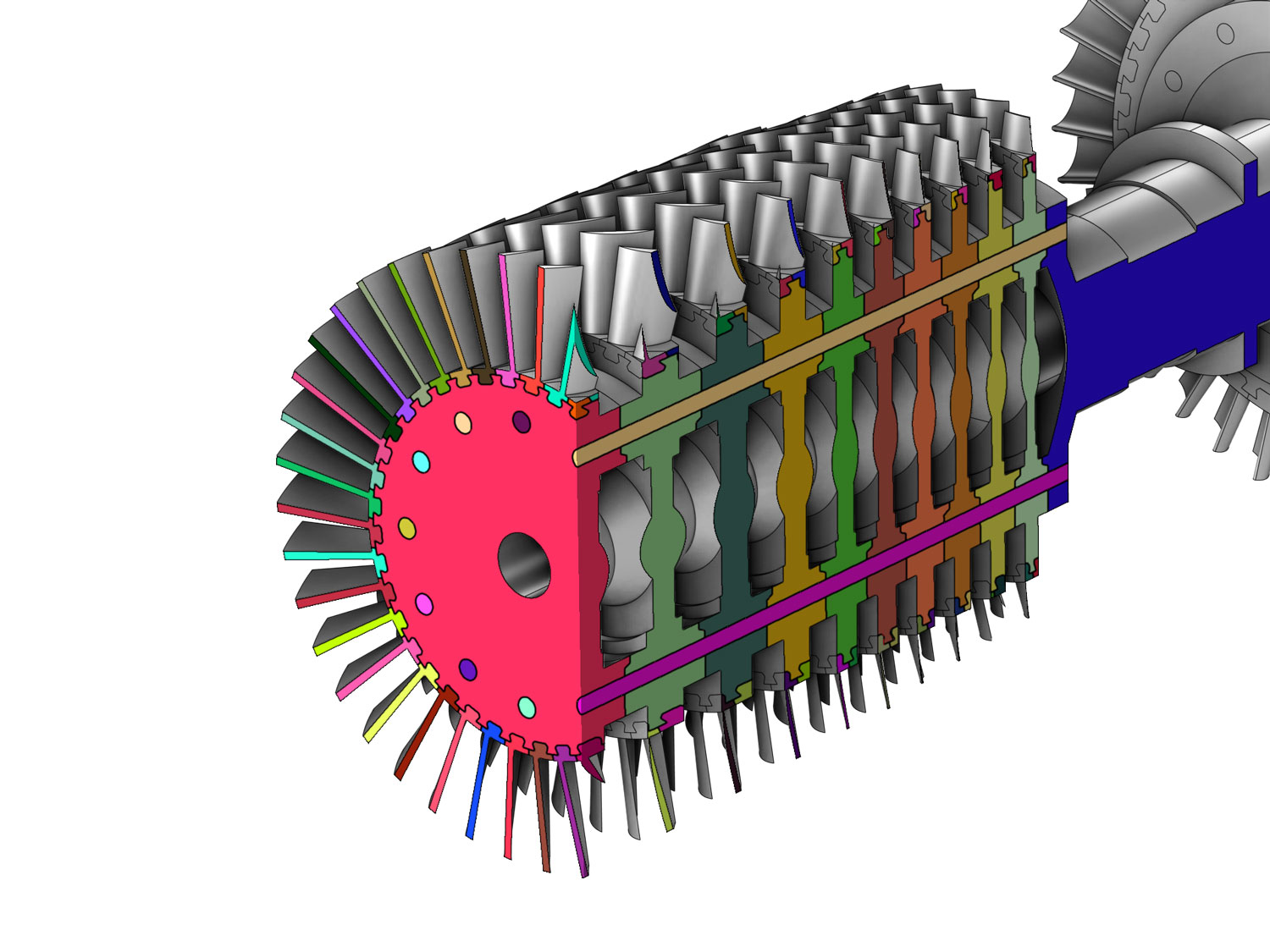
Cross Sections in Interactive Clipping
To make it easier to work with complicated geometries, you can now use the interactive clipping functionality to add cross sections when clipping a solid domain. This feature works throughout the Model Builder and is available from the Graphics window toolbar.
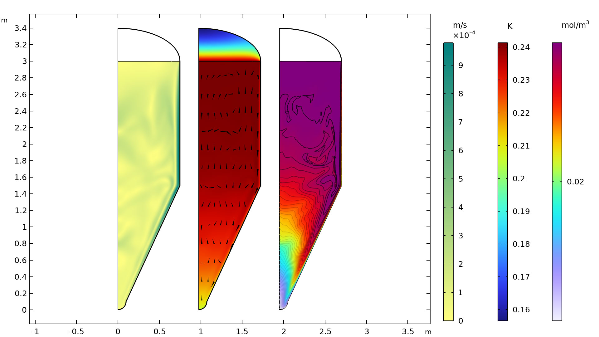
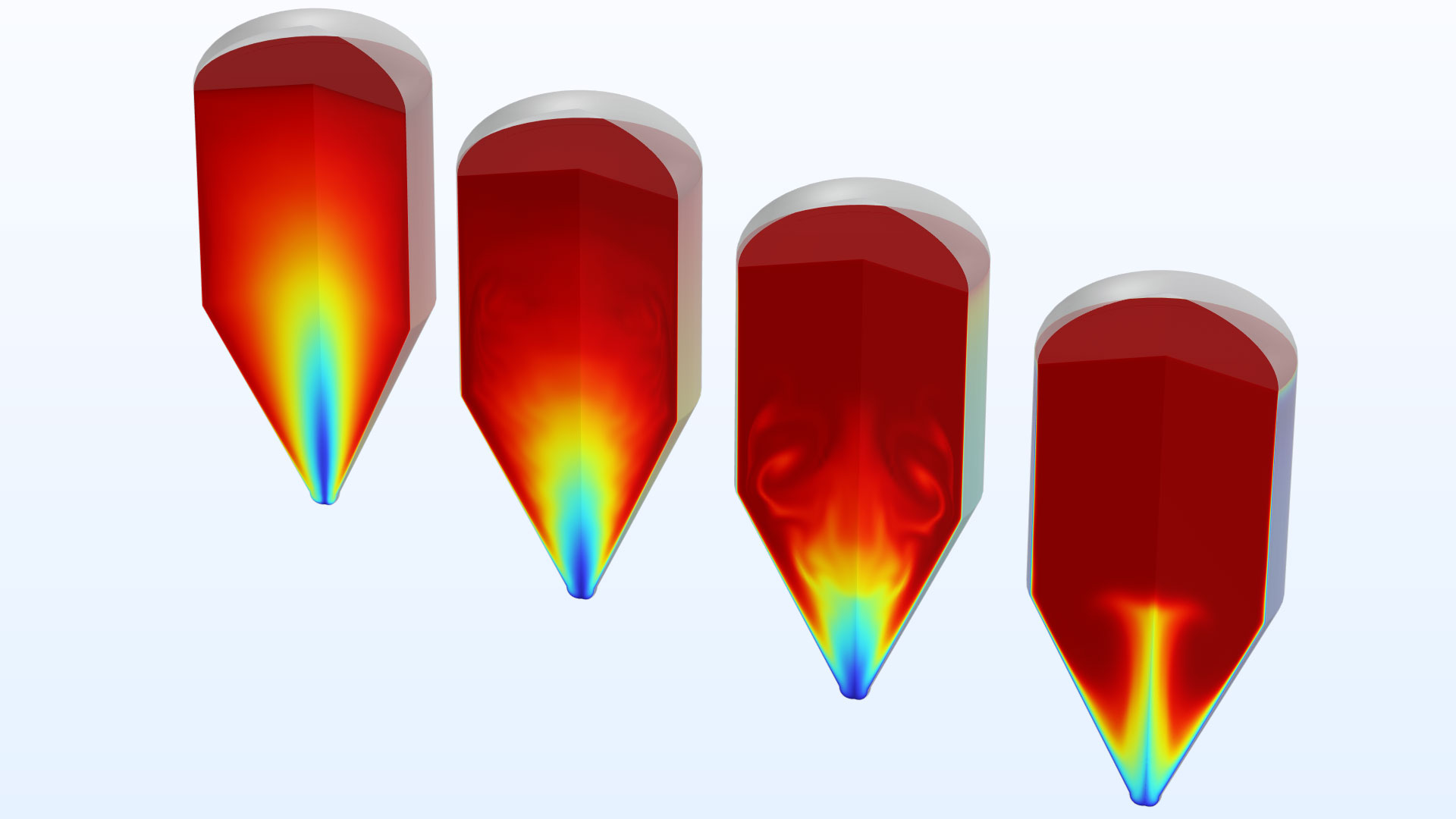
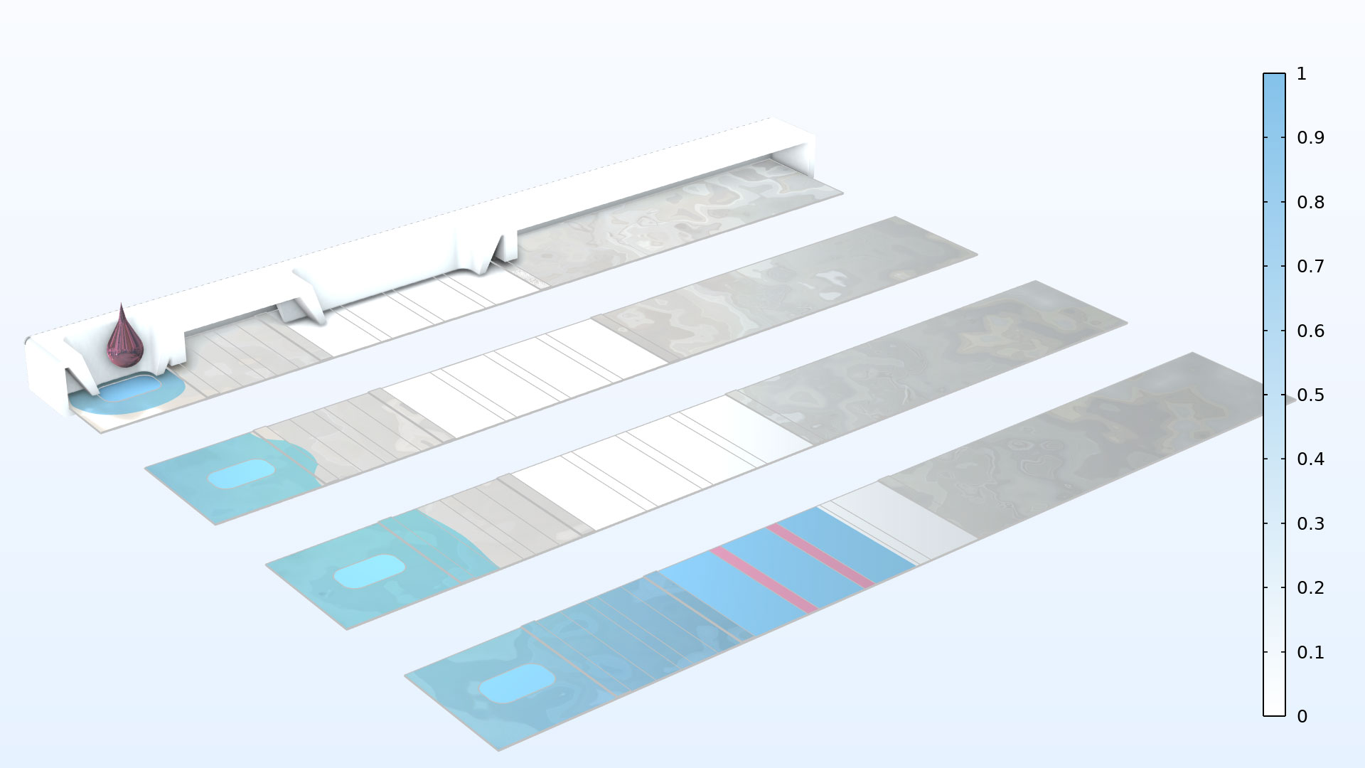
Array of Plots
A new feature allows you to create arrays of plots to visualize multiple results side-by-side in the Graphics window. When the plot array functionality is enabled, you can control the behavior of each plot such as the array shape and array plane in the Settings window under the Plot Array section.
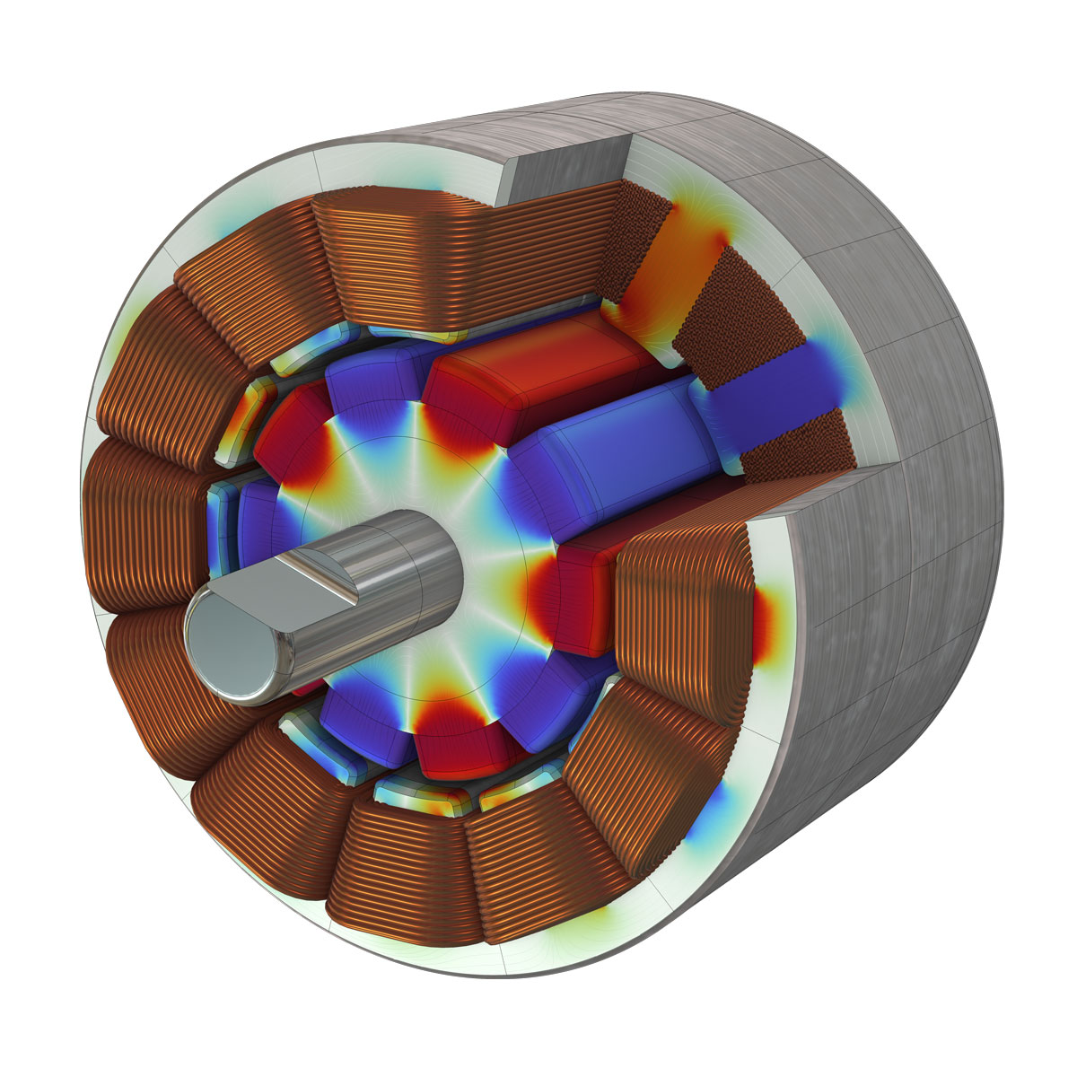
Ambient Lighting Improvements
The Ambient light settings used for providing light around the geometry now includes a new feature to better define 3D models. The new Ambient Occlusion option available in the Graphics window toolbar is a new rendering technique that uses soft shadows to make your geometry appear more realistic. This new feature works by calculating the ambient light exposure of each point in a 3D geometry.

Transparency Improvements
For transparent visualization of plots, transparency can now depend on the incidence angle to help improve realism. In COMSOL Multiphysics® version 6.0, it is now more user friendly to set the mouse rotation center while transparency is enabled.

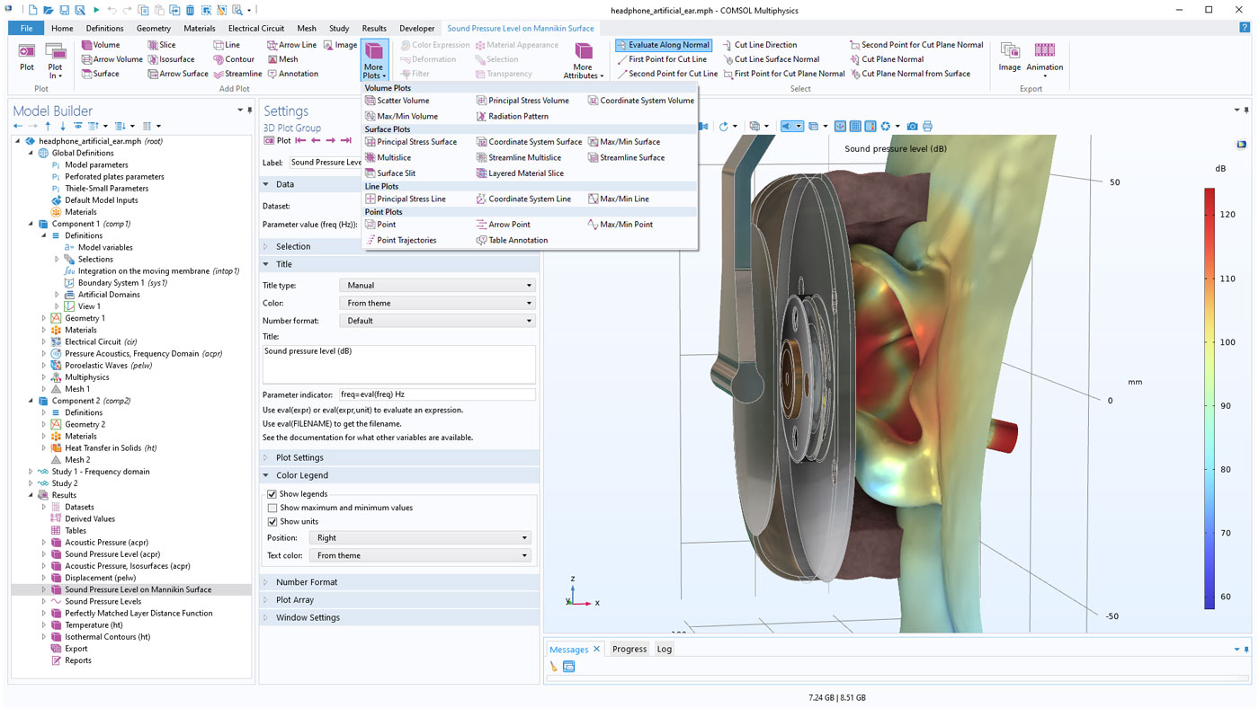
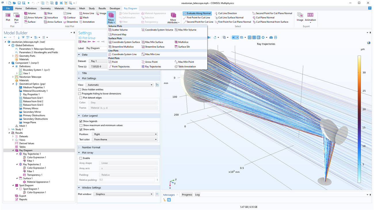
Filtered Lists of Postprocessing Features
The COMSOL® software contains a large number of postprocessing features, but in any given model only a subset of the features is likely to be useful. Version 6.0 brings dynamic filtering in menus based on the physics interfaces that are used in the model. This is especially useful for users who have licenses for many different add-on products.
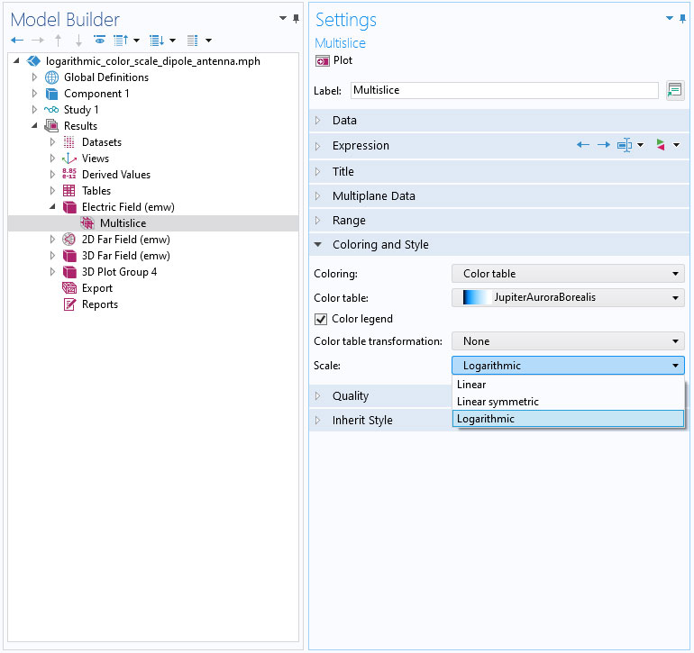
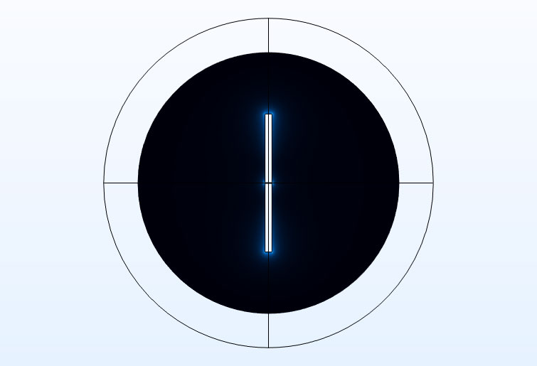
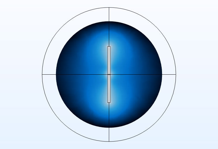
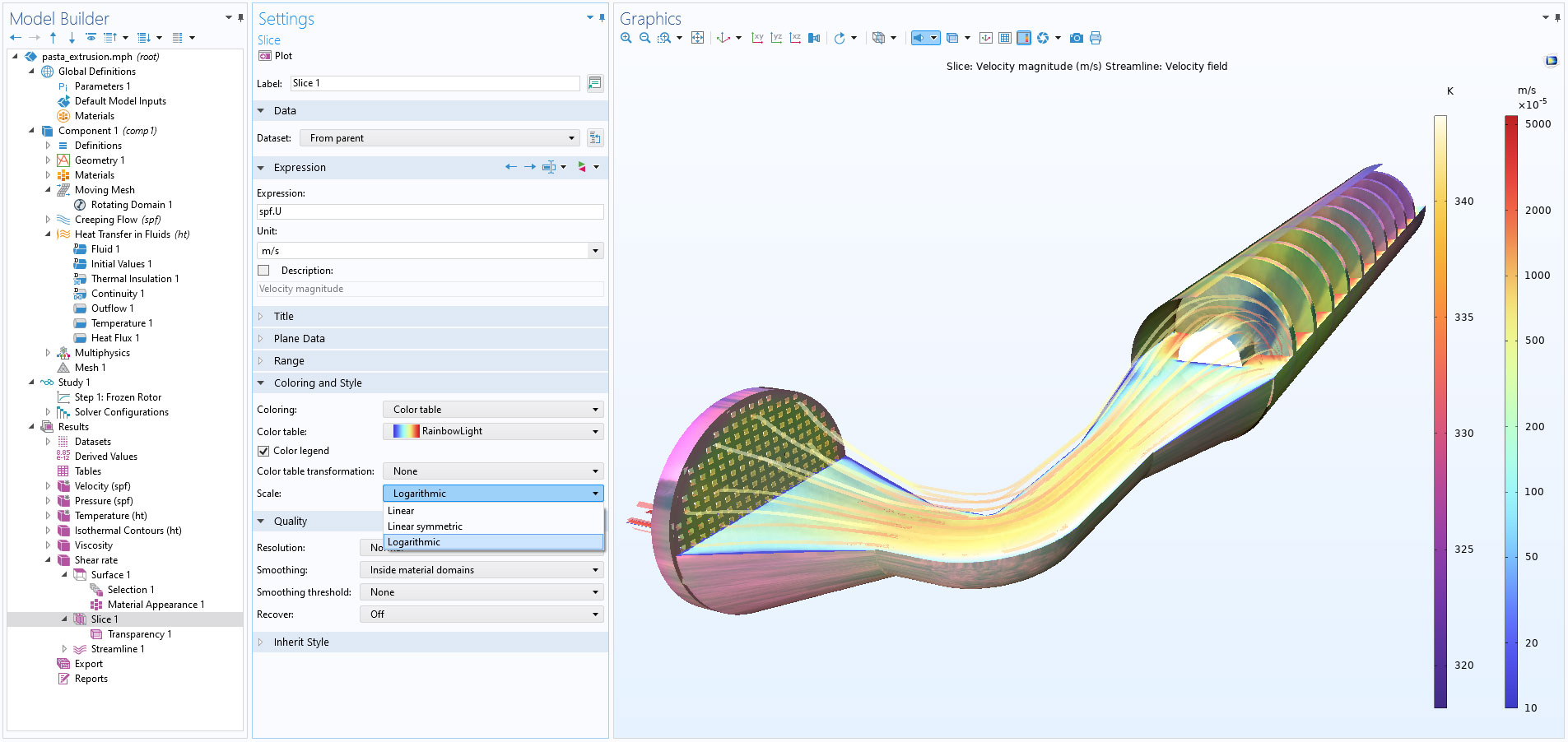
Logarithmic Color Scale
When plotting expressions that have value ranges that cover multiple magnitudes, it can be easier to interpret the results if the logarithm is plotted instead. The obvious way to do this is to plot log(EXPR) or log10(EXPR) instead of EXPR, but doing so has some drawbacks:
- The unit of
EXPRis lost, aslog(EXPR)is dimensionless. - The description of
log(EXPR)does not automatically contain the description ofEXPR. - The values shown next to the color legend are the logarithms.
- The expression has to be changed when changing between linear and logarithmic scales.
In COMSOL Multiphysics® version 6.0, it is possible to use a logarithmic color scale without changing the expression.
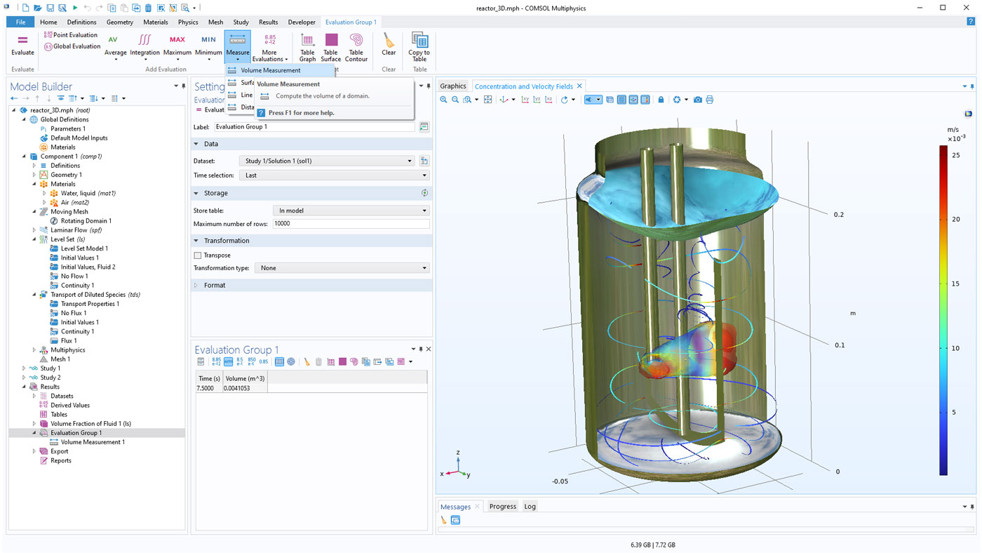
Evaluation of Geometry Measures
The Volume, Surface, Line, and Distance measurement features make it easy to perform measurements in postprocessing. This functionality is analogous to the measure functionality in the geometry sequence.
Cumulative Integration
Cumulative integration can be enabled in the numerical evaluation features in Derived Values and Evaluation Groups. It makes it possible to evaluate cumulative integral values for all time steps.

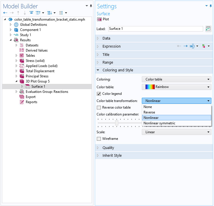
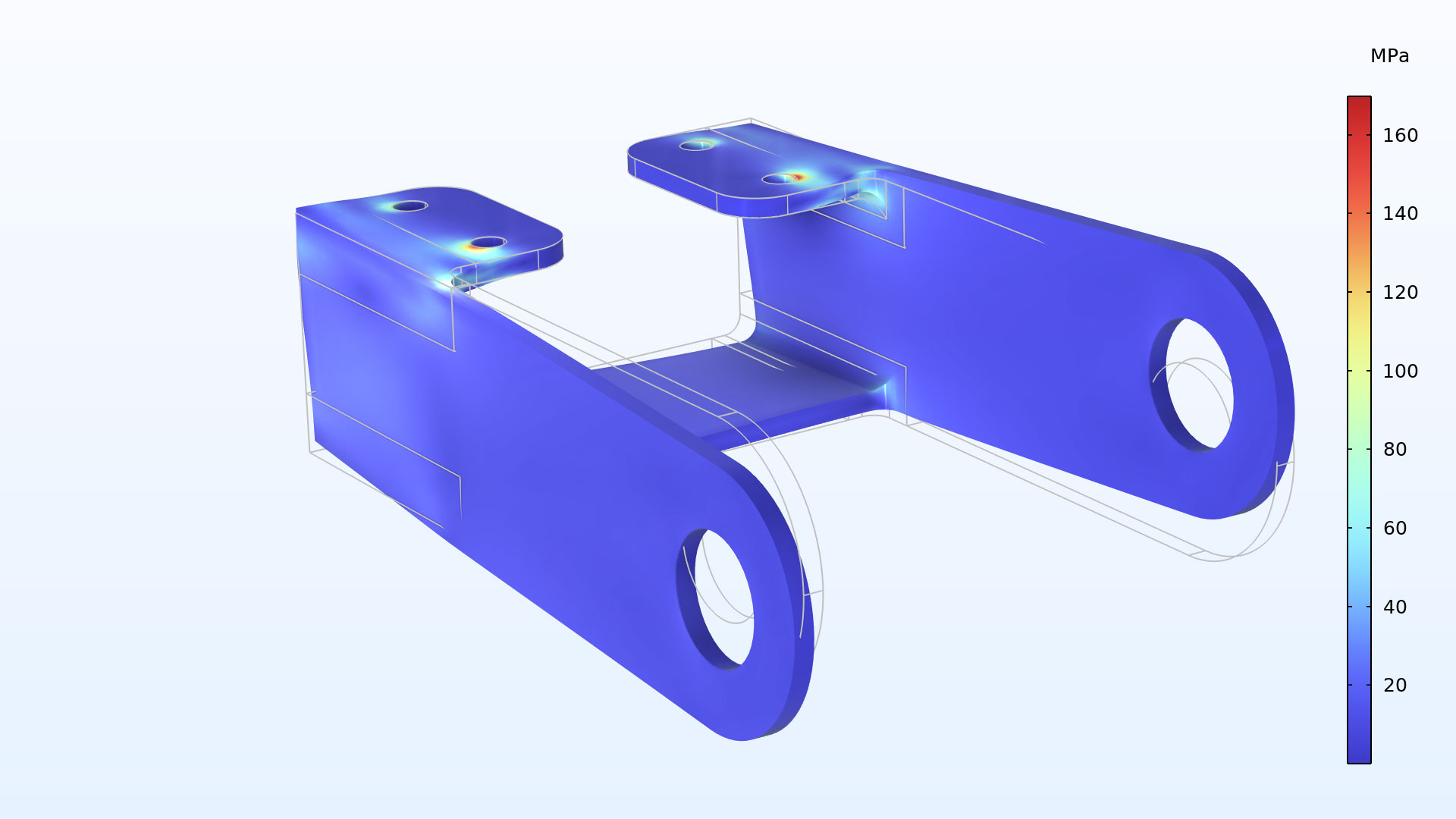
Color Table Transformations
Under the Coloring and Style section, the new Color table transformation options make it possible to tweak a color table by applying a nonlinear transformation to it. You can use this to emphasize or de-emphasize variations in the expressions being plotted.

Transformation Datasets
New Transformation 3D and Transformation 2D datasets make it possible to perform affine transformations of the geometry defined by another dataset. You can use this feature to visualize movements that are not captured by the model's frames or make objects move during an animation, such as in the case of frozen rotor analysis in CFD, for example.
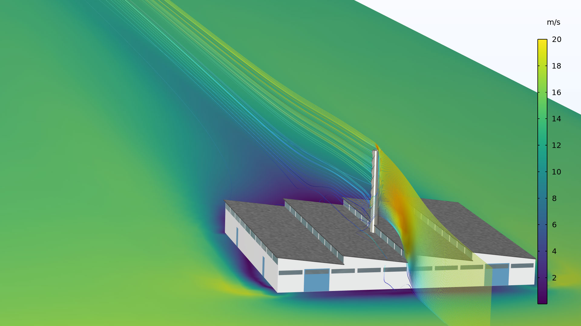
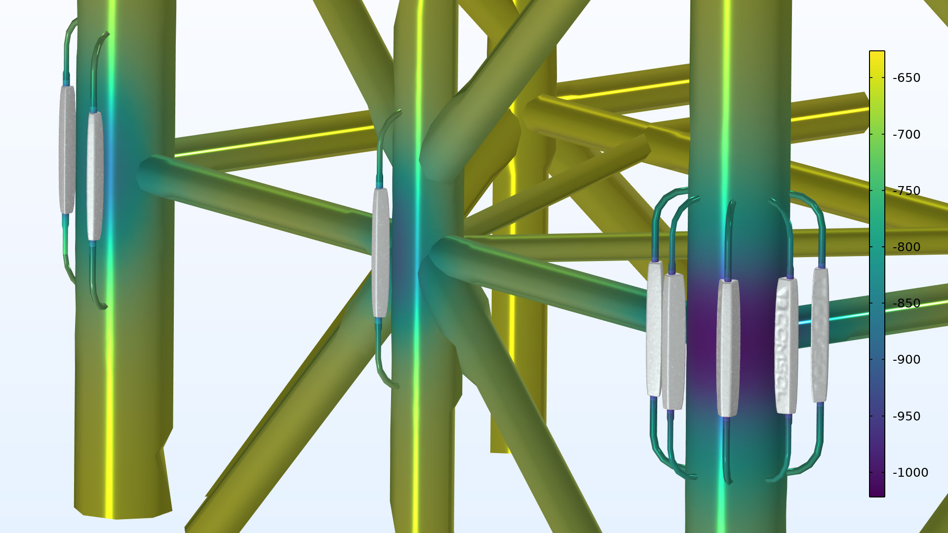
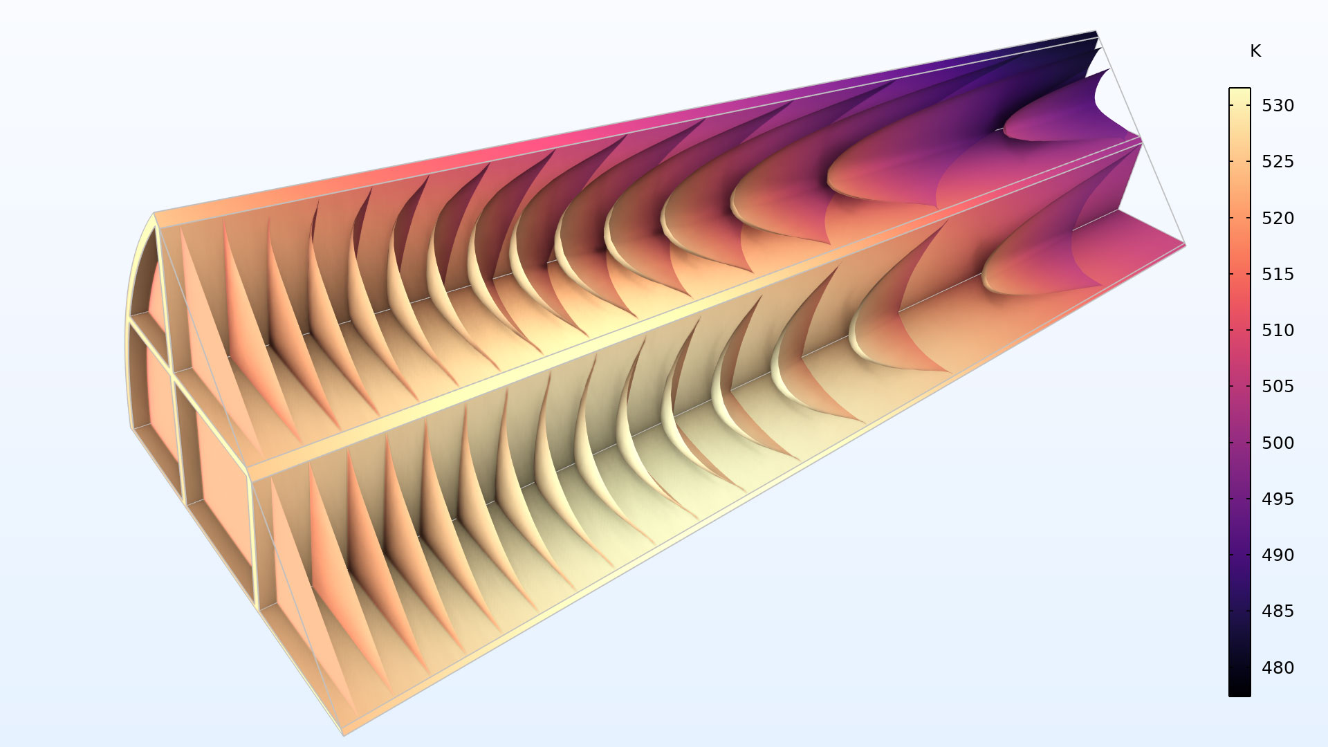
Color Table Improvements
To further enhance your postprocessing, COMSOL Multiphysics® has expanded its range of visualization capabilities by making the color tables smoother and introducing several new color tables, including but not limited to:
- Inferno
- Magma
- Plasma
- ThermalWave
- Viridis
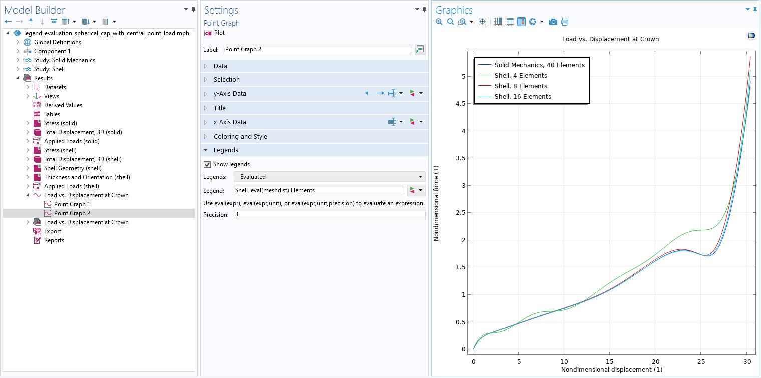
Evaluating Expressions in Graph Plot Legends
A new Evaluated legend type allows you to use the eval function to create an evaluated legend text in the Legend field that includes evaluated global expressions such as global parameters used in sweeps. It is also possible to evaluate expressions defined in the points that are plotted.
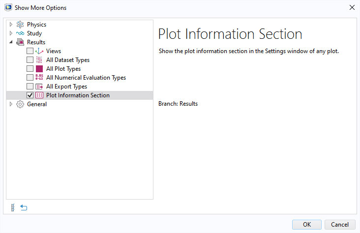
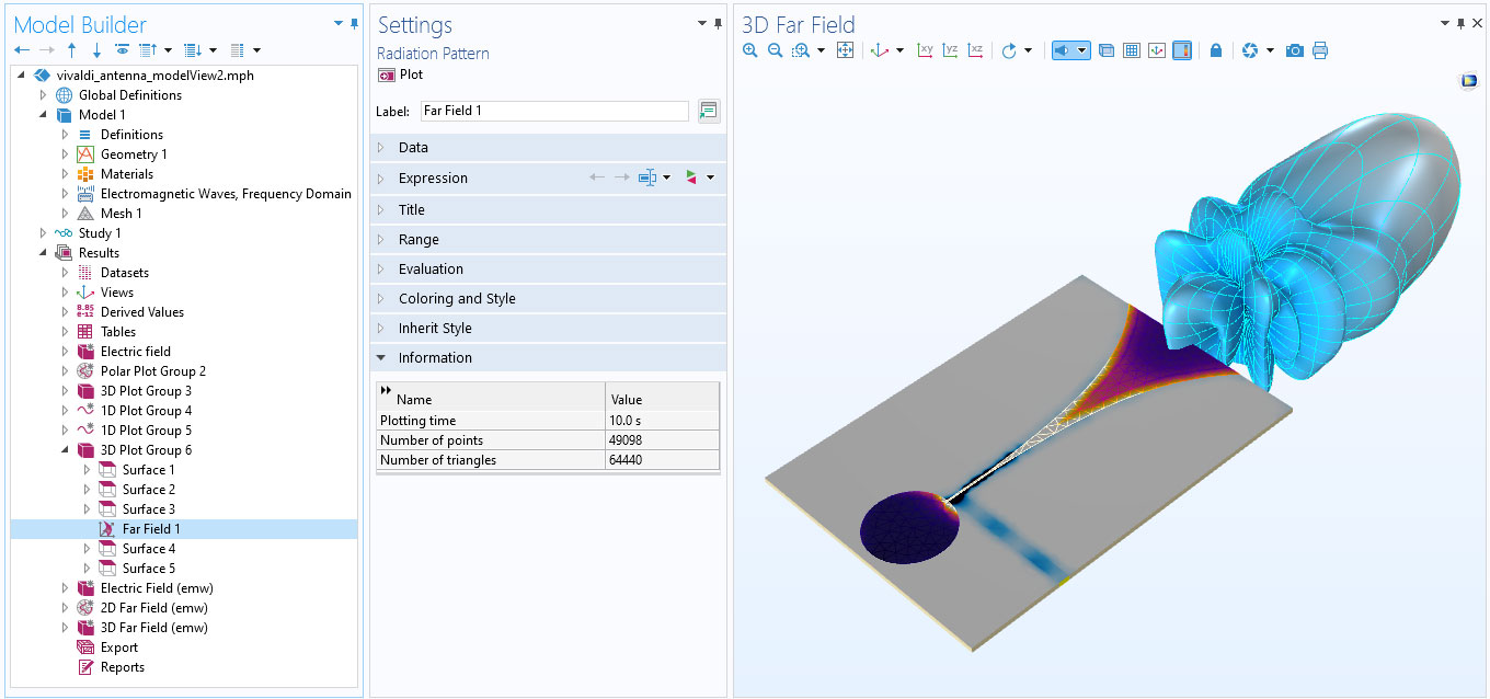
Plot Information Section
There is a new Plot Information Section in the Settings window for all plots and graphs to display different quantities useful for benchmarking against different settings and setups, such as the time that it took to prepare the data for the plot. The information appears in a table that is saved with the model and updated each time the plot had to be redrawn. This section is hidden by default, and you can enable it in the Show More Options dialog box by selecting the Plot Information Section check box.