Particle Tracing Module Updates
For users of the Particle Tracing Module, COMSOL Multiphysics® version 6.0 brings two new tutorial models and many usability improvements, such as the option to transform particle coordinates loaded from a file, as well as faster algorithms to compute the lift and drag force in wall-bounded channel flows. Learn more about these updates below.
New Tutorial Models
Three-Body Problem
The three-body problem involves calculating the positions and velocities of three objects under mutual gravitational attraction, with given initial positions and velocities. While it does not have a general analytic solution, and can display chaotic behavior, certain initial conditions are known to repeat the same configuration periodically. Below is an animation of the figure-eight solution to the three-body problem, which is considered stable because the particle motion remains periodic if the initial conditions are slightly perturbed. In this model, the gravitational force is added as a Particle-Particle Interaction force. You can download the model from the associated Application Gallery entry.
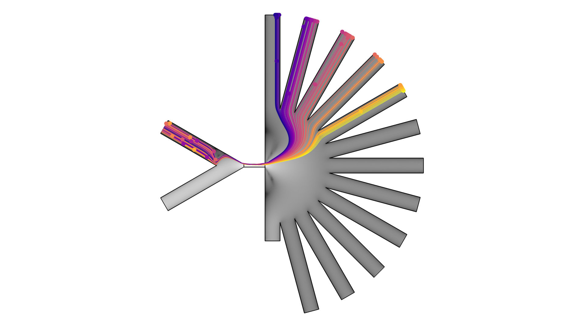
Pinched Flow Fractionation
This tutorial model uses the pinched flow fractionation method to simulate the separation of particles based on their size. First, the Laminar Flow interface is used to calculate the velocity field in a microchannel. Next, the Particle Tracing for Fluid Flow interface is used to calculate the trajectories of injected particles. Histograms are used to track the separation of the particles based on their size and quantify the range of sizes of particles at each outlet. You can download the model from the associated Application Gallery entry.
Simplified Names for Nonlocal Couplings
All particle tracing interfaces define couplings to compute the sum, average, maximum, or minimum of an expression over the particles in a model. In COMSOL Multiphysics® version 6.0, the names of these couplings have been simplified for easier use. You can see this update in the new Three Body Problem model and these existing models and application:
For an instance of the Mathematical Particle Tracing interface (pt), the following table lists the old and new names.
| Coupling Description | Old Name | New Name |
|---|---|---|
| Sum over particles | pt.ptop1(expr) | pt.sum(expr) |
| Sum over all particles | pt.ptop_all1(expr) | pt.sum_all(expr) |
| Average over particles | pt.ptaveop1(expr) | pt.ave(expr) |
| Average over all particles | pt.ptaveop_all1(expr) | pt.ave_all(expr) |
| Maximum over particles | pt.ptmaxop1(expr) | pt.max(expr) |
| Maximum over all particles | pt.ptmaxop_all1(expr) | pt.max_all(expr) |
| Minimum over particles | pt.ptminop1(expr) | pt.min(expr) |
| Minimum over all particles | pt.ptminop_all1(expr) | pt.min_all(expr) |
| Evaluate at maximum over particles | pt.ptmaxop1(expr, evalExpr) | pt.max(expr, evalExpr) |
| Evaluate at maximum over all particles | pt.ptmaxop_all1(expr, evalExpr) | pt.max_all(expr, evalExpr) |
| Evaluate at minimum over particles | pt.ptminop1(expr, evalExpr) | pt.min(expr, evalExpr) |
| Evaluate at minimum over all particles | pt.ptminop_all1(expr, evalExpr) | pt.min_all(expr, evalExpr) |
The old names will continue to work in version 6.0 as well, so it is not necessary to update any existing models.
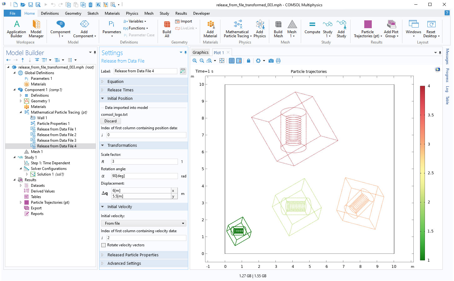
Transformations when Loading Particle Positions from a File
When you use the Release from Data File node to load the initial particle positions from a file, you can now apply Transformations to the initial coordinates. You can use any combination of dilation (scaling), rotation, and translation. Optionally, if the initial particle velocity is also loaded from a file, you can apply the same rotation to both the position and velocity.
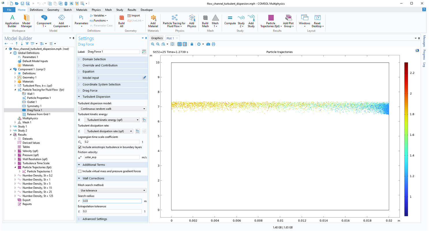
Fast Boundary Search for Wall-Induced Lift and Drag
In the Particle Tracing for Fluid Flow interface, the lift force, drag force, and anisotropic turbulent dispersion for wall-bounded flows are now faster to evaluate with new options for setting up the search for the nearest boundary element to each particle. You can now choose between the Closest point (the default behavior, and the only behavior in version 5.6) or faster options, Use tolerance and Walk in connected component where you can specify the maximum search radius. This is a useful option for particle tracing in pipes and channels with very high aspect ratios. You can see this new feature in the existing Dispersion of Heavy Particles in a Turbulent Channel Flow tutorial model.
Accumulate Dose from Energetic Ion Bombardment
When modeling the passage of energetic ions through solid matter, you can now accumulate the absorbed dose and dose equivalent in the domain as the ions pass through in the Particle-Matter Interactions node. You can choose to compute the accumulated dose by selecting any combination of the check boxes Absorbed dose, Absorbed dose from ionization losses, or Absorbed dose from nuclear stopping.

Heat Transfer Between Particles and Surrounding Fluid
You can now calculate the heat transfer between particles and surrounding fluid using the new Dissipated Particle Heat feature. The particles can be used as heat source/sink for the surrounding fluid. To use this feature, you need to check the Compute particle temperature in the Particle Tracing for Fluid Flow interface and use the Convective Heat Losses feature to calculate the heat flow rate from particles.
Convective cooling of hot particles settling in a fluid. The surface plot shows the temperature in the fluid due to dissipated heat from the particles.