MEMS Module Updates
For users of the MEMS Module, COMSOL Multiphysics® version 5.6 brings enhanced electrostriction functionality and improved tutorial models. Browse all of the MEMS updates below.
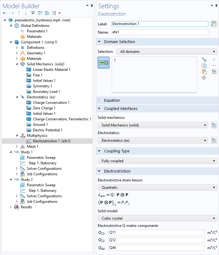
Electrostriction Multiphysics Interface
The functionality for modeling electrostriction was previously available in the Electromechanical Forces multiphysics coupling node. That functionality has been significantly enhanced and moved into a new Electrostriction multiphysics interface. This interface consists of the Solid Mechanics and Electrostatics interfaces, together with the new Electrostriction multiphysics coupling. In Electrostatics, the standard Charge Conservation material model is used. You can add and use the new feature by itself or use it together with the Electromechanical Forces node, if needed. For existing models that use the old electrostriction functionality, a new Electrostriction node will be added automatically when opening the model.
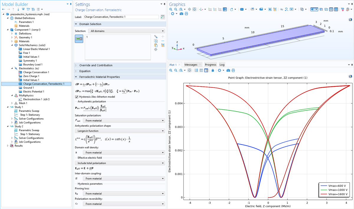
Ferroelectroelasticity Multiphysics Interface
A new Ferroelectroelasticity multiphysics interface is intended for analysis of ferroelectric materials exhibiting nonlinear piezoelectric properties. This multiphysics interface will add Solid Mechanics and Electrostatics interfaces, together with the new Electrostriction multiphysics coupling. In Electrostatics, the new Charge Conservation, Ferroelectric material model is used to simulate, for example, hysteresis using a Jiles–Atherton model. You can see this interface used in the new Hysteresis in Piezoelectric Ceramics tutorial model.
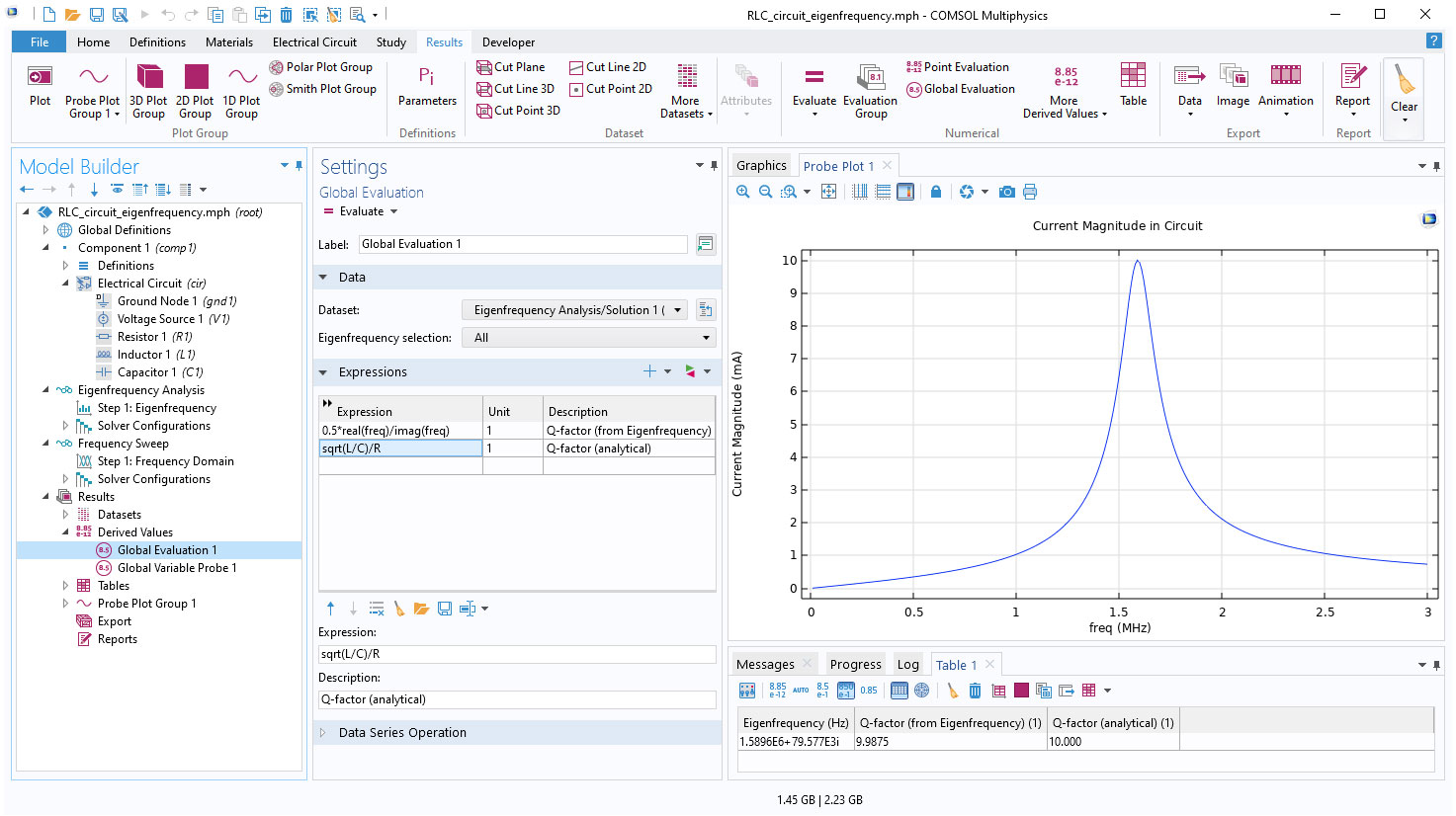
Wide Support for Eigenfrequency Analysis
The Eigenfrequency study is now supported for most of the AC/DC Module interfaces: Electric Currents, Electric Currents in Shells, Electric Currents in Layered Shells, Electrical Circuit, Electrostatics, and Magnetic Fields. In addition to supporting full-wave cavity mode analysis in the Magnetic Fields interface, it is possible to run eigenfrequency analyses with models involving electrical circuits. The eigenfrequency support is primarily developed for the AC/DC Module, but other modules that provide one of the affected physics interfaces will benefit from it too.
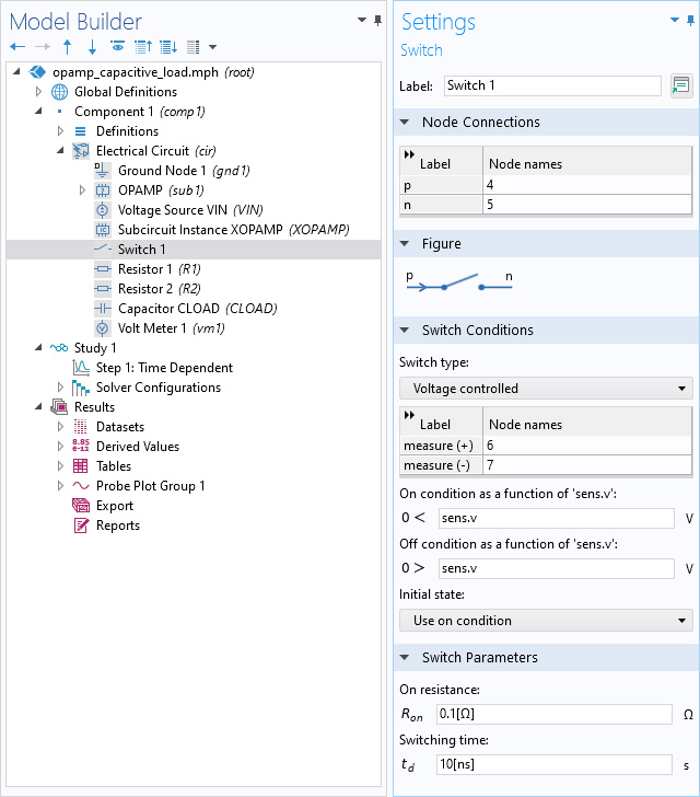
New and Enhanced Functionality for the Electrical Circuit Interface
For Time Dependent studies, the Electrical Circuit interface has been equipped with an "event-based" Switch feature. This allows you to model the "instantaneous" on-off switching of certain connections in the circuit. The switch can be current controlled, voltage controlled, or controlled by user-defined Boolean expressions.
Furthermore, Parameterized Subcircuit Definitions are added. Together with the Subcircuit Instance, these allow you to create your own building blocks containing smaller circuits, and use multiple parameterized variants of those in your larger circuit. Finally, the state, event, and solver machinery has been improved, especially the transient modeling of nonlinear (semiconductor) devices, which has become more robust.
The circuit improvements are primarily developed for the AC/DC Module, but other modules that provide access to the Electrical Circuit interface will benefit too. You can view the new functionality in these updated models:
- operational_amplifier_with_capacitive_load
- battery_over_-_discharge_protection_using_shunt_resistances
- p_-_n_diode_circuit
- reverse_recovery_of_a_pin_diode
Dynamic Contact
New algorithms for dynamic contact provide a significant improvement of the conservation of momentum and energy during transient contact events. This means that you can accurately model transient contact problems with significantly larger time steps than in previous versions. The new methods are accessed by selecting either the Penalty, dynamic or Augmented Lagrangian, dynamic formulation in the Contact node. You can see this functionality in the new Impact Between Two Soft Rings and Impact Analysis of a Golf Ball tutorial models.
Springs and Dampers Connecting Points
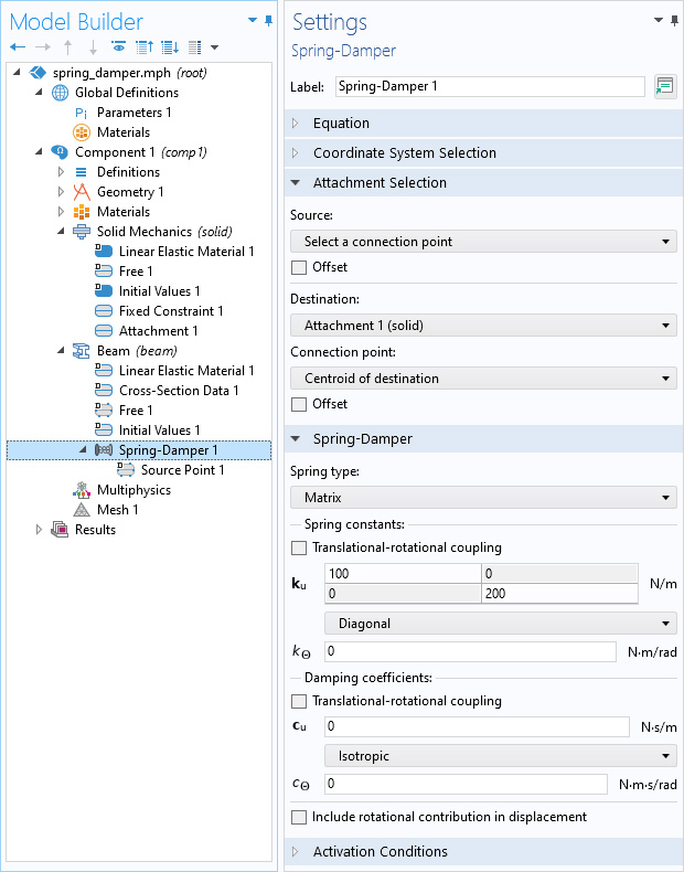
In all structural mechanics interfaces, a new feature called Spring-Damper has been added to connect two points with a spring and/or damper. The points can be geometrical points, but they can also be abstract, for example, through the use of attachments or direct connections to rigid bodies. The spring can either be physical, with a force acting along the line between the two points, or described by a full matrix, connecting all translational and rotational degrees of freedom in the two points. The feature also makes it possible to connect a spring between points in two different physics interfaces.
Port Boundary Condition for Elastic Wave Propagation
The new Port boundary condition, available with the Solid Mechanics interface, is designed to excite and absorb elastic waves that enter or leave solid waveguide structures. A given Port condition supports one specific propagating mode. Combining several Port conditions on the same boundary allows a consistent treatment of a mixture of propagating waves, for example, longitudinal, torsional, and transverse modes. The combined setup with several Port conditions provides a superior nonreflecting condition for waveguides to a perfectly matched layer (PML) configuration or the Low-Reflecting Boundary feature, for example. The port condition supports S-parameter (scattering parameter) calculation, but it can also be used as a source to just excite a system. The power of reflected and transmitted waves is available in postprocessing. To compute and identify the propagating modes, the Boundary Mode Analysis study is available in combination with the port conditions. You can view this functionality in the new Mechanical Multiport System: Elastic Wave Propagation in a Small Aluminum Plate tutorial model.

Rigid Connector Improvements
The Rigid Connector features have multiple improvements. In the Shell and Beam interfaces, the selection alternatives have been extended to the top level, that is, boundaries and edges, respectively. When the center of rotation is defined by a point selection, the point no longer has to be part of the physics interface itself. You can couple rigid connectors from different physics interfaces, thus defining a new type of virtual rigid object (this selection resides in the Advanced section of the settings for the rigid connector). In the Solid Mechanics, Shell, and Beam interfaces, you can automatically generate rigid connectors from RBE2 elements in an imported file in the NASTRAN® format. This is controlled from a section named Automatic Modeling in the settings for these interfaces. Rigid connectors can belong to several physics interfaces, in order to mimic the connections in the imported file.
New Option for Prescribing Rotating Frame Speed
In the Rotating Frame node in the Solid Mechanics and Multibody Dynamics interfaces, a new Rigid body option has been added. With this option, you enter a time-dependent torque around the axis of rotation, and the rotational velocity is computed by integration of the rigid body equation of motion.
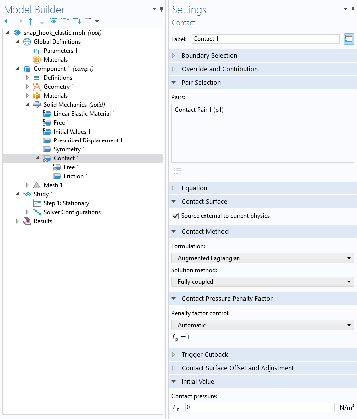
Contact Improvements
In addition to the new dynamic contact and wear functionality, there are several other improvements in the field of contact mechanics. You can use a fully coupled solver together with the augmented Lagrangian contact algorithm, making it easier to set up solver sequences and improving stability and convergence for some problems. Also, in the Friction subnode under Contact, you can select User defined as the Friction model to directly enter an expression for the tangential force that causes sliding in terms of any other variables. Lastly, there are several new ways of providing penalty factors, both for the penalty method and for the augmented Lagrangian method.
Viscoelasticity Improvements
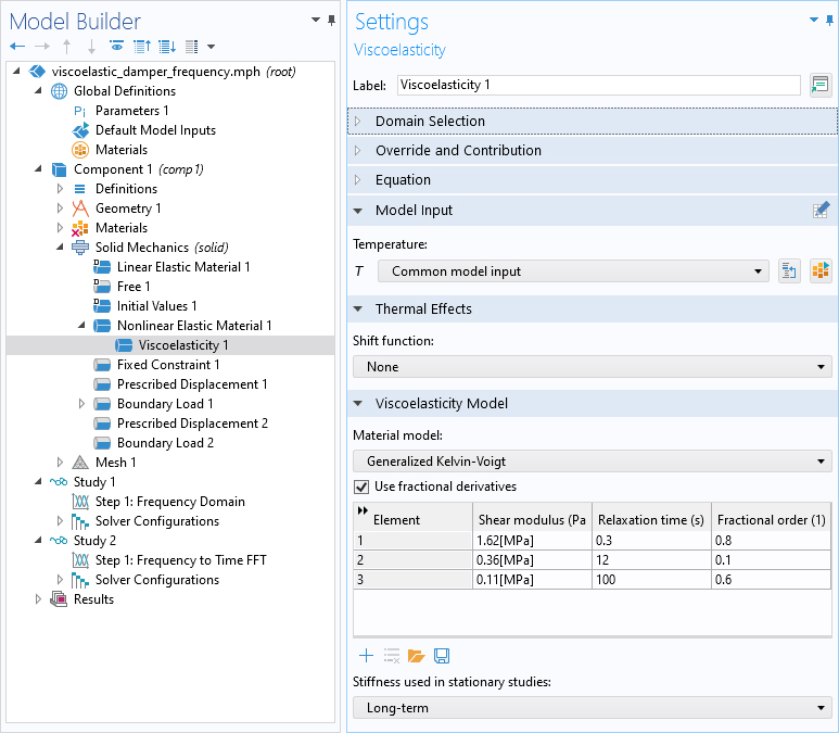
Two new viscoelasticity models have been added: Maxwell and Generalized Kelvin-Voigt. The Maxwell material can be considered as a type of liquid, since its long-term deformation under a constant stress is unbounded. The Generalized Kelvin-Voigt model has a Prony series representation with several time constants. Conceptually, it consists of a set of Kelvin elements (spring and dashpot elements in parallel) connected in series.
For frequency-domain analyses, all of the viscoelasticity models (Generalized Maxwell, Generalized Kelvin-Voigt, Maxwell, Kelvin-Voigt, Standard Linear Solid, and Burgers) have been augmented by a fractional derivative representation. Using a fractional time derivative representation makes it easier to fit material data to experiments for some materials. For time-domain analyses using the Generalized Maxwell and Standard Linear Solid viscoelastic models, performance has been improved by up to one order of magnitude.
The Tool–Narayanaswamy–Moynihan shift function is commonly used to describe the glass transition temperature in glasses and polymers. It has been added to the set of shift functions in the Viscoelasticity node.
New Settings for Solving Transient Elastic Wave Problems with Solid Mechanics
New settings have been introduced in the Solid Mechanics interface that ensure a correct and efficient solver setup when solving elastic wave problems in the time domain. The settings are similar to the existing settings in the transient acoustics interfaces. In the Solid Mechanics interface node, a new Transient Solver Settings section has been introduced with an option to specify the Maximum frequency to resolve. This should be the maximum frequency content of the source's excitation or the maximum eigenmode frequency that can be excited. The automatically generated solver suggestion will have settings that use an appropriate solver method for wave propagation and ensure proper resolution in both time and space.
Improved Models
The Thin-Film BAW Composite Resonator model has been updated in several respects. To improve the performance of the perfectly matched layer (PML) domain condition, the PML scaling, curvature, and mesh are adjusted to cover longer wavelengths. The typical wave speed is made consistent across material boundaries. Additionally, the region search method for the eigenfrequency is used to avoid spurious solutions.
The Piezoelectric Rate Gyroscope model has been updated with a simplified geometry and refined mesh. Additionally, the Eigenfrequency study has been updated to solve for the full system, which is consistent with the Frequency Domain studies.
The Electrostrictive Disc model has been updated to include the new Ferroelectroelasticity functionality.
New Tutorial Models
COMSOL Multiphysics® version 5.6 brings several new tutorial models to the MEMS Module.
Hysteresis in Piezoelectric Ceramics
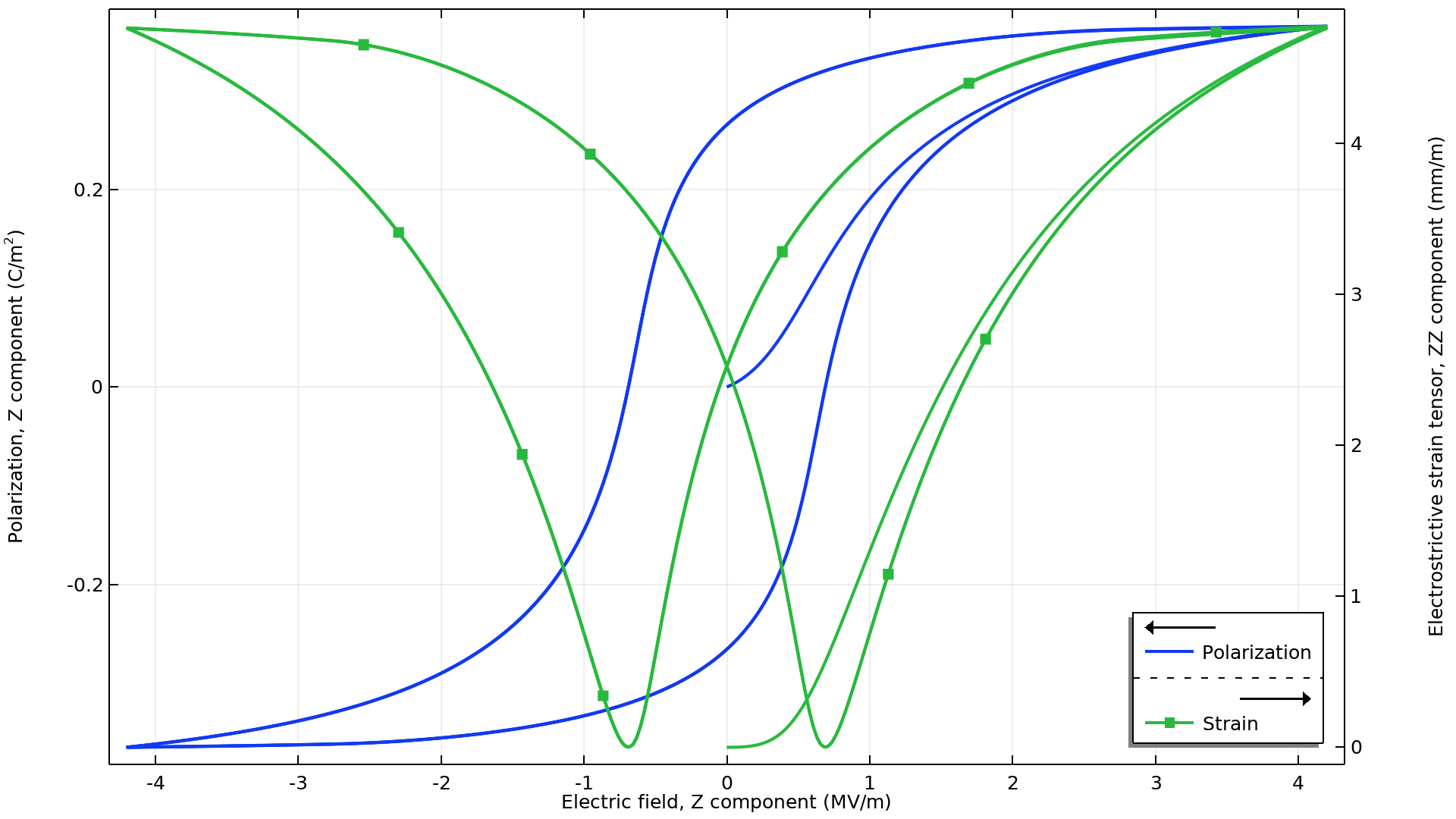
Application Library Title:
piezoelectric_hysteresis
A Micromachined Comb-Drive Tuning Fork Rate Gyroscope
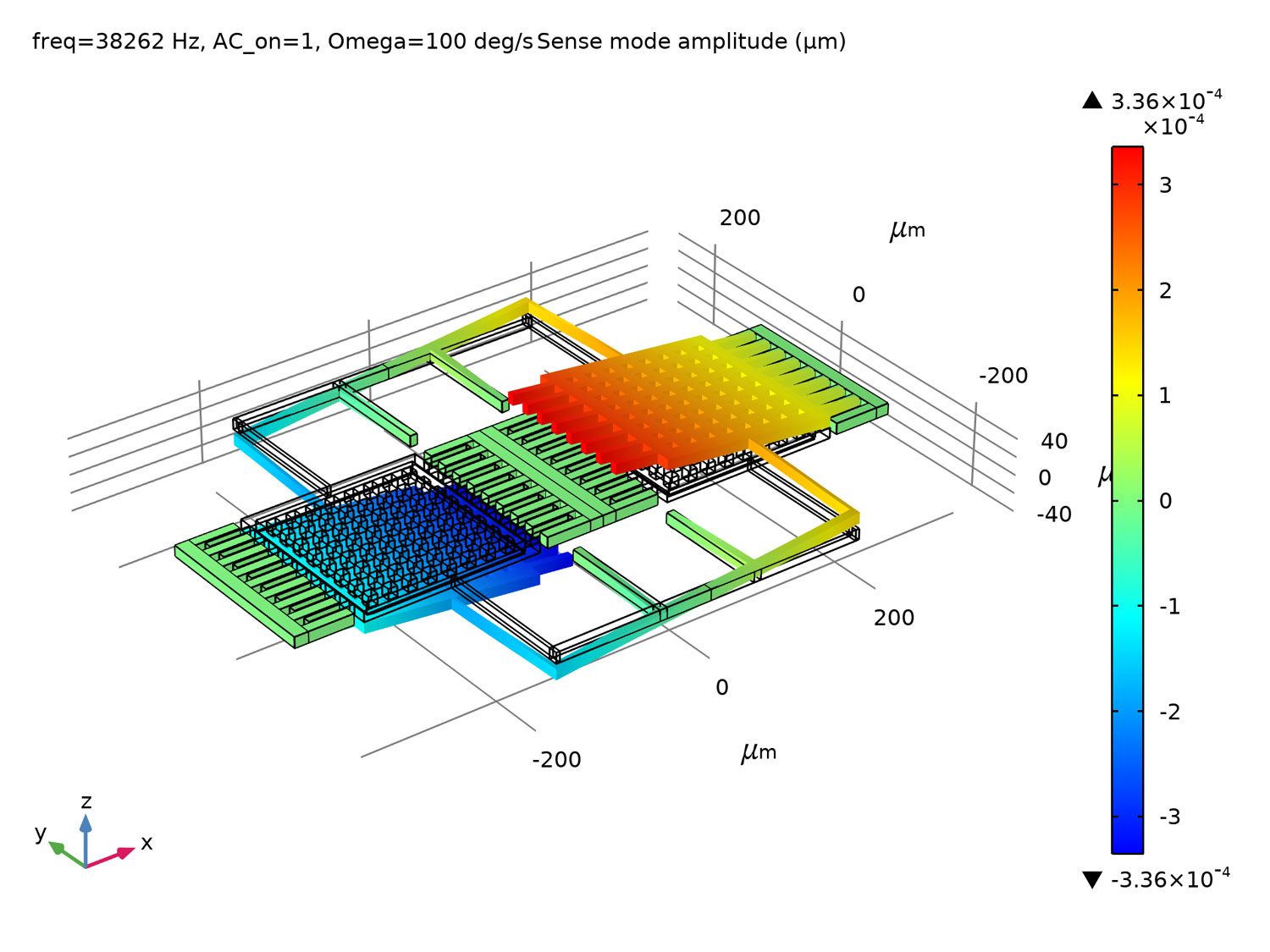
Application Library Title:
comb_drive_tuning_fork_gyroscope
A Piezoelectric Micropump
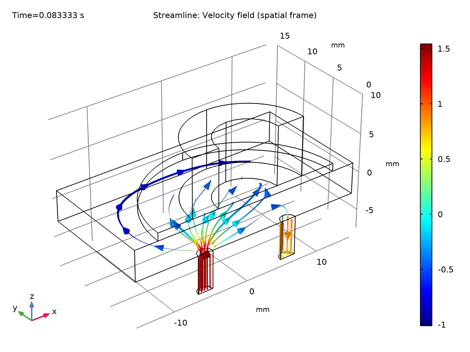
Application Library Title:
piezoelectric_micropump
Manufacturing Variation Effects in a Micromachined Comb-Drive Tuning Fork Rate Gyroscope
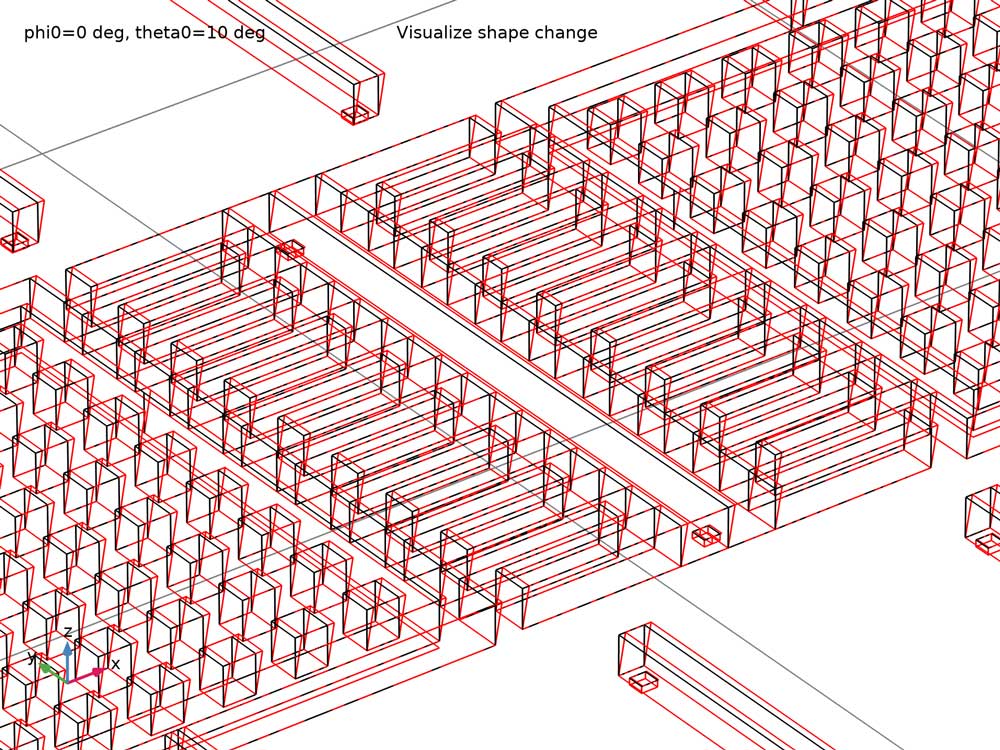
Application Library Title:
comb_drive_tuning_fork_gyroscope_manufacturing_variation