
You can perform response spectrum analyses with a study type introduced in version 5.4 of the COMSOL Multiphysics® software. In this blog post, we will give an introduction to how you can analyze a structure subjected to a short transient excitation being described by a response spectrum.
What Is Response Spectrum Analysis?
Response spectrum analysis is used to determine the maximum value of displacements, stresses, or any other result quantity in a structure during a short transient event. The loading must be a synchronous acceleration of all points connected to a common base. The method has its origins in earthquake engineering, which is still an important application today.

A building destroyed by the 2010 earthquake in Haiti. Image by Master Sgt. Jeremy Lock — United States Air Force and in the public domain via Wikimedia Commons.
Aside from earthquake mechanics, shock response spectrum analysis is also used on a smaller scale. For instance, it is a common requirement that electronic equipment contains a specified response spectrum. In this case, it can be shocks from impact during transportation, which is the targeted transient event.
What such events have in common is that the actual time history of the anticipated excitation is not known. The duration of the event is short, so it is not possible to perform an analysis based on the statistical properties of an input signal, as you would do in a random response analysis.
A response spectrum analysis is based on a superposition of eigenmodes, and it assumes that the response of the structure is predominantly linear.
The Fundamental Idea Behind Response Spectrum Analysis
The input to a shock response analysis is a response spectrum, which contains an amplitude as function of the frequency. The response spectrum actually shows how a simple system with a single degree of freedom would respond to a given base acceleration.
Find the full theory behind shock response spectrum analysis here.
For each eigenfrequency of the structure, the corresponding value from the response spectrum is multiplied with the modal participation factor in order to determine the peak displacement of that mode when excited in a certain direction. An important aspect is that such modal peak values cannot just be summed up, because not all modes reach their peak value at the same time. A pure summation would provide certain upper bounds, but for most real structures, the predictions will be so pessimistic that they are not usable. The core of response spectrum analysis is the different methods by which the modes are combined in order to estimate the total peak response.
Analyzing Shock Response Spectra in COMSOL Multiphysics®
When you are performing a response spectrum in COMSOL Multiphysics, the core of the computations is actually done on the fly during the result evaluations. The study is an ordinary eigenfrequency study, and all response-spectrum-specific settings are done using a special dataset. When you add a response spectrum study from the Add Study window, two things will happen:
- A study with an Eigenfrequency study step will be added
- A Response Spectrum node will be added under Definitions
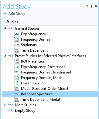
Adding a Response Spectrum study.
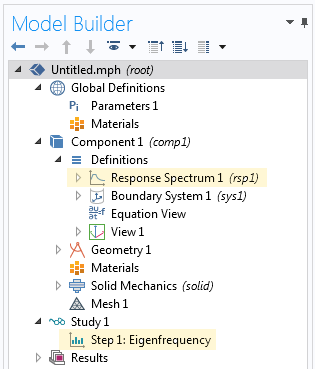
Two nodes are added to the Model Builder tree.
The Eigenfrequency study step is fairly standard. Some default values have been changed for convenience, but you can actually use any eigenfrequency study step as a basis for response spectrum analysis. Moreover, a separate eigenfrequency analysis is often the first step in the study of any vibrating structure. If you already have a suitable solved eigenfrequency study in your model, there is no need to add a new Response Spectrum study; you can just manually add the Response Spectrum node under Definitions.
So, what does the Response Spectrum node do? Its purpose is to define several variables (mainly, the modal participation factors and modal masses) needed during postprocessing. There are some possible settings in the node, but they are only interesting when working with missing mass correction — an option which will be discussed later.
Once you have computed the eigenfrequencies, you can add one or more Response Spectrum 2D or Response Spectrum 3D datasets, depending on the dimensionality of your component.
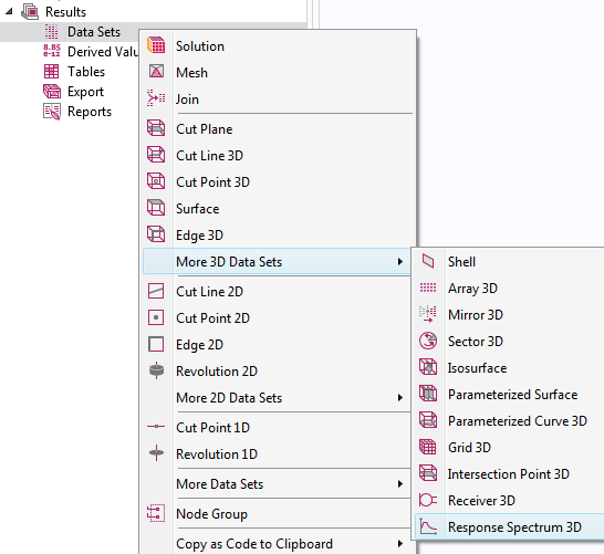
Adding a dataset for response spectrum evaluation.
There is a multitude of settings for the response spectrum datasets that we will go over, but you can start by selecting the relevant eigenfrequency solution in the Data section.
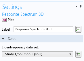
Selecting the dataset containing eigenfrequency results.
Finding the Response Spectrum
The load input for a response spectrum analysis is sometimes called a design response spectrum. From the perspective of the analyst, the spectrum can, in most cases, be considered as given; for example, in a building design code. For the case of earthquake engineering, the design response spectrum to be used can depend on the geographical location, as well as on the local soil properties.
A response spectrum is valid for a certain level of structural damping, usually around 5%. Since the damping information is provided by the response spectrum, no damping should be added in material models or other features in the physics interface.
A design response spectrum can be provided either as a function of frequency or as a function of period time. The values of the spectrum are provided in terms of displacement, (pseudo-)velocity, or (pseudo-)acceleration. The most fundamental input, and the one that is actually used to scale the eigenmodes, is the displacement spectrum.
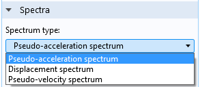
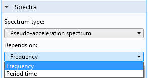
Selecting the type of design response spectrum and its definition.
To enter a response spectrum, you add it as a function under Global Definitions.

Example of an acceleration response spectrum; here as function of period time.
It is common that a response spectrum is specified by a graph consisting of straight lines in a log-log diagram. If you use an interpolation function to describe it, you need to add many points between the break points in the original graph to get the correct interpolation. Alternatively, you can add a piecewise function and use the analytical description of the response spectrum.
Depending on the type of event you are studying, the spectrum to be used may differ with spatial directions. For earthquakes, it is common to assume different spectra in the horizontal and vertical directions, whereas for impact simulation, it is more common to use the same spectrum in all directions.
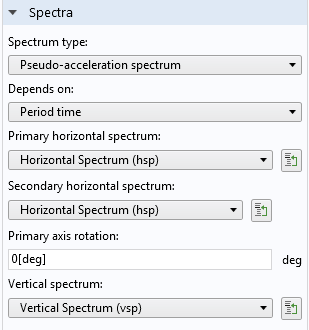
Selection of the response spectrum functions in a 3D dataset.
It is assumed that the vertical direction corresponds to global Z in 3D, and to global Y in 2D. In 3D, you can supply different spectra in two horizontal directions. By default, the primary spectrum is applied along the global X-axis. However, by entering the Primary axis rotation angle, you can choose any other orientation. When the two horizontal spectra are not the same, you often need to test several rotation angles in order to find the worst case for a certain result quantity.
Combination Methods for the Eigenmodes
The core of the response spectrum method is the algorithm used to combine the modes. In most methods, the combination is performed in two passes. The response due to excitation in each of the spatial directions is computed in the first pass. In a second pass, the results for the three (or two) directions are then combined.
The default mode combination method is a complete quadratic combination (CQC). It is a modern, theoretically well-founded method. However, several other methods are also in common use.
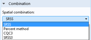
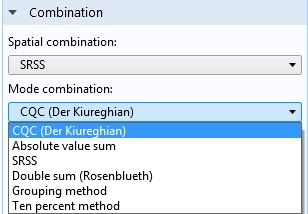
Specification of combination methods.
Each combination method comes with its own set of settings.
The CQC3 or SRSS3 methods are special. In these methods, the spatial and modal combination are performed simultaneously. Here, you cannot select a separate mode combination method. These two methods are very efficient when the secondary horizontal spectrum is the same as the primary horizontal spectrum, except for a scale factor.
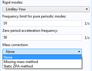
Sometimes, it is required to separate the responses from the individual modes into what is termed as periodic and rigid modes. The idea is that modes with a high frequency (relative to the frequency content of the excitation) are classified as rigid. Such modes will, to a large extent, be synchronous with the excitation, and thus with each other. These modes will then reach their peak values at the same time, which contradicts the summation principles used above. To incorporate this effect, you can choose between two methods: Gupta and Lindley-Yow.

Selecting a method for separating periodic and rigid modes.
The original theory behind the CQC3 and SRSS3 methods deals only with periodic modes, but in COMSOL Multiphysics, there is an implemented extension so that all combination methods can coexist with the Gupta and Lindley-Yow methods.
Missing Mass Correction
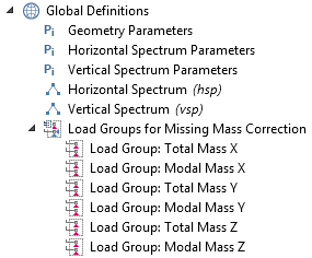
As with any method based on mode superposition, the true response of a structure is approximated through the response of a limited number of modes. This means that some part of the true load is lost, since it would have been applied to the omitted modes. For the case of response spectrum analysis, the load actually represents a homogeneous acceleration in each spatial direction. Because of this, each mode can be considered to have a certain fraction of the total mass attributed to it. This is the modal mass. Thus, it is actually easy to see how large of a fraction of the true load is missing: Sum up the modal masses for all modes and compare it with the total mass of the structure. These variables are readily accessible.
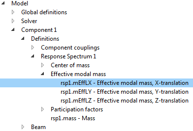
Variables created by the Response Spectrum node.
If the part of the mass not accounted for is significant, it can be important to compensate for it. Thus, some standards require that a missing mass correction must be used if less than 90% of the total mass is accounted for. The missing mass belongs to the high-frequency modes that were not used in the analysis. Since such modes essentially follow the base excitation without amplification, the response to the missing mass can be considered stationary. In order to perform a missing mass correction, you need to solve for a set of extra stationary load cases. Setting up that analysis manually would be rather cumbersome, but fortunately it is automated.
Let’s go back to the Response Spectrum node, where you will find a button for setting up the missing mass correction study.
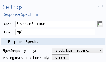
The Response Spectrum node.
First, you need to select the appropriate eigenfrequency study, so that the missing mass computation can be connected to the correct eigenmodes. After that, you can click the Create button, which triggers the following modifications in the model:
Step 1
A number of load groups is created under Global Definitions.
Step 2
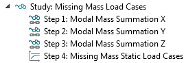
A special study sequence is created. The first three study steps are used to compute the distribution of the missing mass, and finally, the load cases are solved in a stationary study.
Step 3
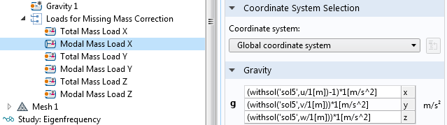
Under all structural mechanics interfaces, specially tailored gravity loads are added. They represent the distribution of the missing mass and are assigned to the previously defined load cases.
After this preparation, you can just run the new study sequence.
If you have chosen to use rigid modes in the response spectrum dataset, you can also select a method for the missing mass correction. The missing mass method is the primary choice (and the only one that can be used together with the Gupta method for rigid modes).
Selecting a mass correction method.
When you have chosen to include missing mass correction, the Data section will contain one more entry: Missing mass load cases data set. There, you select the stationary study used for computing the stationary load cases.
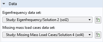
Selection of a dataset for the stationary solution.
Displaying the Shock Response Results
In most nodes under Results, you can select a response spectrum dataset. You can, for example, use plots, graphs, and derived values to present the results of the response spectrum evaluation.
You can evaluate any expression, not only the built-in variables. This differentiates COMSOL Multiphysics from most other software providing a response spectrum analysis capability. For example, you can directly compute a combination of the axial force and bending moment in a beam.
The way the response spectrum evaluation works is that the variable or expression is evaluated for each eigenmode, and the resulting values are then summed up according to the selected combination rules. The combination has certain effects that you should be aware of:
- Since the combination rules contain either squares or absolute values, all signs are lost and the result values are positive. The true peak value can, however, be either positive or negative.
- If you evaluate for example two displacement components,
uandv, the sum of the results does not match what you would get if you evaluateu+v. - Any vector quantity is meaningless, since all three components would be always evaluated positive. Only the values of each individual component have a meaning.
- Consequently, the deformation plots are meaningless, since they are based on the displacement vector evaluation.
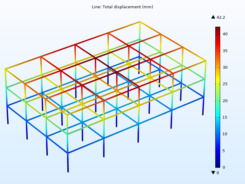
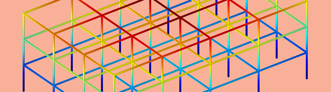
Peak displacements in a building’s steel frame subjected to an earthquake.
A Note on Performance
All results are computed on the fly when you redraw a plot, compute a derived value, or perform a similar operation. Such computations can take a substantial amount of time for large models. Actually, the computation time is almost proportional to the square of the number of eigenmodes used in the analysis. Selecting only those modes that give a significant contribution to the final result can speed up the result evaluation by orders of magnitude.
An example of how that can be done in a systematical way can be found in the Earthquake Analysis of a Building tutorial model. In that model, there are 532 eigenmodes in the frequency range of interest. However, only 20 of them are used in the response spectrum analysis. The salient feature here is the possibility to add a Combine Solutions study step as a filter after the Eigenfrequency study step.
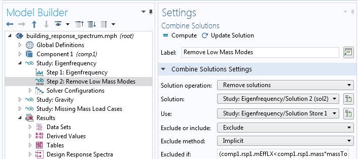
Using Combine Solutions to filter out significant modes.
Next Steps
Learn more about the features and functionality available in the Structural Mechanics Module:
To learn more about how to set up a response spectrum analysis, you can download the following models.


Comments (4)
Enrico Borellini
August 19, 2021Hi.
If I plot the axial stress on the column, all pillar are in traction (not in compression). Why ? Is there a problem into the model ?
Henrik Sönnerlind
August 20, 2021 COMSOL EmployeeBy definition, all result quantities from a response spectrum analysis are without sign. They are computed by ‘square root of sum of squares’ type expressions. You can see the math on our Cyclopedia page, https://www.comsol.com/multiphysics/response-spectrum-analysis
Josh Thomas
January 25, 2022Hi Henrik,
Any reason these Response Spectrum analyses could not be done on a model with shells + solids + shell to solid connections?
Thanks,
Josh Thomas
Henrik Sönnerlind
January 25, 2022 COMSOL EmployeeNo. If you have encountered a problem, please contact support.