

All structural engineers use Saint-Venant’s principle, whether actively or subconsciously. You can find various formulations of this principle in most structural mechanics textbooks, but its exact meaning is not obvious. Saint-Venant’s principle tells us that the exact distribution of a load is not important far away from the loaded region, as long as the resultants of the load are correct. In this blog post, we will explore Saint-Venant’s principle, particularly in the context of finite element (FE) analysis.
The History of Saint-Venant’s Principle
The French scientist Barré de Saint-Venant formulated his famous principle in 1855, but it was more of an observation than a strict mathematical statement:
“If the forces acting on a small portion of the surface of an elastic body are replaced by another statically equivalent system of forces acting on the same portion of the surface, this redistribution of loading produces substantial changes in the stresses locally, but has a negligible effect on the stresses at distances which are large in comparison with the linear dimensions of the surface on which the forces are changed.”
B. Saint-Venant, Mém. savants étrangers, vol. 14, 1855.
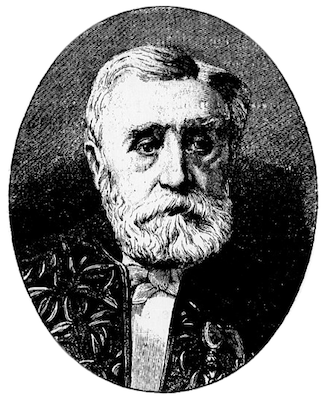
Portrait of Saint-Venant. Image in the public domain, via Wikimedia Commons.
Many great minds within the field of applied mechanics — Boussinesq, Love, von Mises, Toupin, and others — were involved in stating Saint-Venant’s principle in a more exact form and providing mathematical proofs for it. As it turns out, this is quite difficult for more general cases, and research on the topic is still ongoing. (The argumentation has at times been quite vivid.)
Simple Example: Analyzing Stresses at a Distance
Let’s start with something quite simple: a thin rectangular plate with a circular hole at some distance from the loaded edge, which is being pulled axially. If we are interested in the stress concentration at the hole, then how important is the actual load distribution?
Three different load types are applied at the rightmost boundary:
- A constant axial stress of 100 MPa
- A symmetric parabolic stress distribution with peak amplitude 150 MPa
- A centered point load with the same resultant as the two previous load cases
As seen in the plots below, the stress distribution at the hole is not affected by how the load is applied. The key here is, of course, that the hole is far enough from the load.
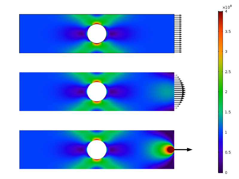
Von Mises stress contours for the three load cases.
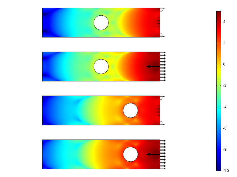
Another way of visualizing this scenario is by using principal stress arrows. Such a plot emphasizes the stress field as a flux and gives a good feeling for the redistribution.
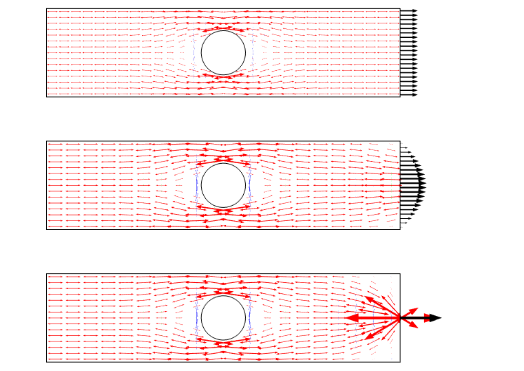
Principal stress plot for the three load cases. Note that there is a singularity when a point load is used.
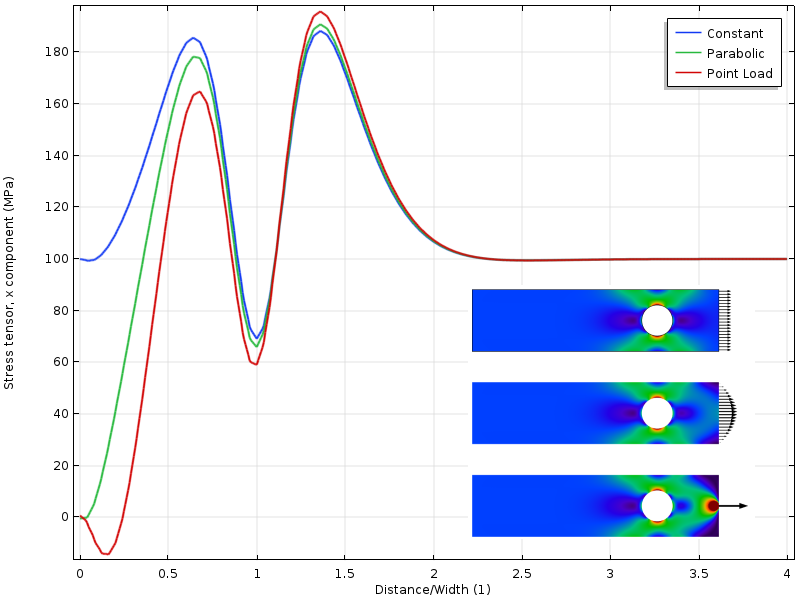
By graphing the stress along a line, we can see that all three cases converge to each other at a distance from the edge, which is approximately equal to the width of the plate.
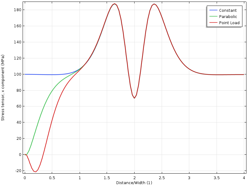
Stress along the upper edge as a function of the distance from the loaded boundary. The distance is normalized by the width of the plate.
If the hole is moved closer to the loaded boundary, we get another situation. The stress state around the hole now depends on the load distribution. But even more interesting is that the distance to where the three stress fields agree now is twice as far from the loaded boundary. The application of Saint-Venant’s principle requires that the stresses are free to redistribute. In this case, that redistribution is partially blocked by the hole.
Stress along the upper edge with the hole closer to the loaded boundary.
Note that Saint-Venant’s principle tells us that there is no difference in the stress state at a distance that is of the order of the linear dimension of the loaded area. The loaded area to be taken into consideration, however, may not be the area that is actually loaded! This statement may sound strange, but think of it this way: When the hole is far away, we may compute the stress concentration factor using a handbook (mine says 4.32) rather than by an FE solution. The handbook approach contains an implicit assumption that the load is evenly distributed as in the first load case. So even if the actual load was applied to only a small part of the boundary, the critical distance in that case is related to the size of the whole boundary.
When solving the problem using the finite element method (FEM), then the hole can be arbitrarily close to the load. What sets the limit is that from the physical point of view, the load distribution is well defined. As soon as we make assumptions about redistribution, however, there is an implicit assumption about the load distribution, which may differ from the actual one.
Zero Resultant Systems and Strain Energy Density
So far, we have said that the stresses are the same independent of the load details at some suitable distance. Since we are dealing with linear elasticity here, it is always possible to superimpose load cases. When working with proofs of Saint-Venant’s principle, it is easier to formulate a principle along these lines: The stresses caused by a load system with no resulting force or moment will be small at a distance that is of the same order of magnitude as the size of the loaded boundary.
Thus, we study the stress caused by the difference between the two load systems with equal resultants. Most modern proofs are based on estimates of the decay of the strain energy density for such a zero-resultant system.
Returning to the problem above, we can compute the difference between the load cases. Doing so allows us to study the actual decay of stress or strain energy density for the difference of the stress fields.
Logarithm of strain energy density for the zero-resultant load cases.
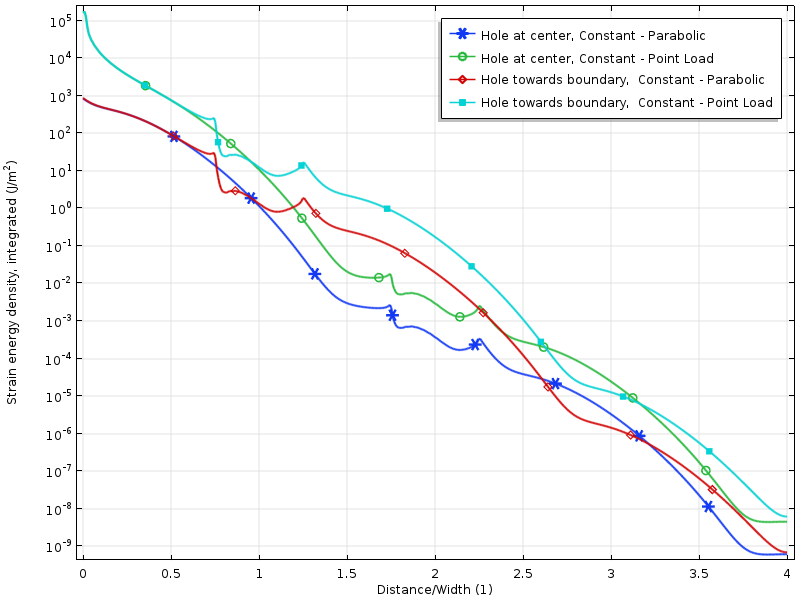
The strain energy density along the plate for the zero resultant load cases. The energy is integrated along the vertical direction in order to produce a quantity that is only a function of the distance from the load.
The decay in the logarithm of the strain energy density is more or less linear with the distance from the loaded boundary. This is actually in line with what modern proofs predict: an exponential decay of the strain energy density. We can also clearly see how the hole temporarily reduces the decay rate.
Applying Saint-Venant’s Principle to Thin Structures
For thinner structures like shells, beams, and trusses, it is well known that Saint-Venant’s principle cannot be applied the same way as for a more “solid” object. Disturbances travel longer distances than what we expect, because the load paths in a thin structure are much more limited. This is the same phenomenon we see with the hole in the example above, but more prominently.
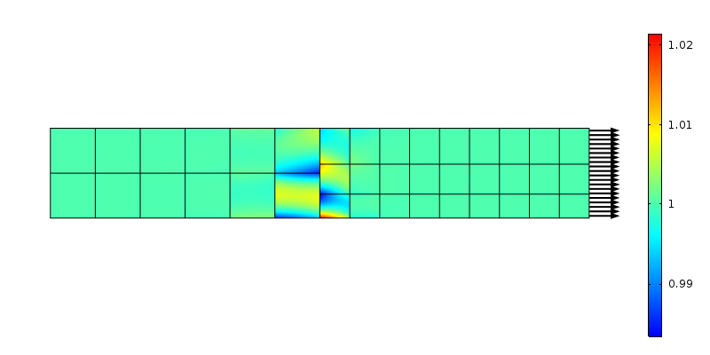
Here, we study a beam with a standard IPE100 cross section. The end of the beam is subjected to an axial stress, with an amplitude that has a linear distribution in both cross-sectional directions.
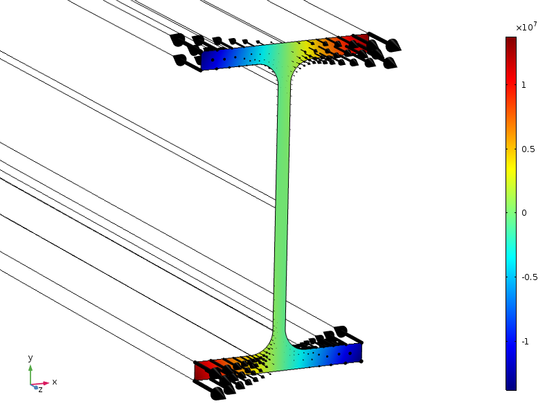
Load distribution, displayed as contours and arrows.
Due to the symmetries, this load has a zero-resultant force, as well as zero moment around all axes. The height of the cross section is 100 mm, so if the standard form of Saint-Venant’s principle is applicable, then the stresses should be small at a distance of approximately 100 mm from the end section.
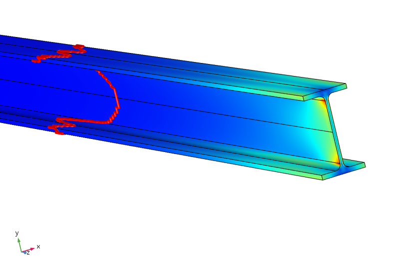
Equivalent stress in the beam. The red contour indicates where the stress is less than 5% of the peak applied stress.
It turns out that in order for the stress to be below 5% of the peak applied stress, we have to travel almost a meter along the beam. Thus, the load redistribution is much less efficient here, since the equilibration between the top and bottom flanges requires moment transfer through the thin web.
If you are familiar with the theory for nonuniform torsion of beams (i.e., warping theory or Vlasov theory), you will recognize that the applied load has a significant bimoment. The bimoment is a cross-sectional quantity with the physical dimension force X length2.
Maybe (this is just my personal speculation), an efficient Saint-Venant’s principle for this case should require not only force and moment but also a bimoment of zero. This can be accomplished by adding four point loads that provide a counteracting bimoment. The result of such an analysis is shown below.
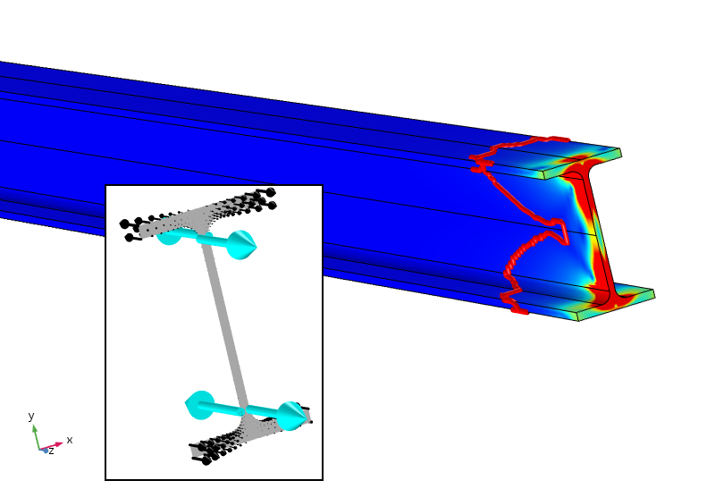
Equivalent stress with four point loads that also provide a zero bimoment. The 5% stress contour is now much closer to the loaded boundary.
The applied point loads, which are not optimally placed on purpose, give extremely high (actually singular) local stresses. However, the stress does drop off much faster and is below 5% after about 100 mm. The 5% limit is still in terms of the applied distributed load, so it is not adjusted for the new local stresses. The logarithmic decay rate of the strain energy density is three times faster after the point loads are added.
Saint-Venant’s Principle in Finite Element Analysis
In some cases, you can intuitively consider Saint-Venant’s principle to be applicable to the FE discretized problem. Here, we look at distributed loads and nonconforming meshes.
Distributed Loads
In the FE model, loads are always applied at the mesh nodes, even though you specify them as a continuous boundary load. The load is internally distributed to the nodes of the element using the principle of virtual work, as shown in the example below.
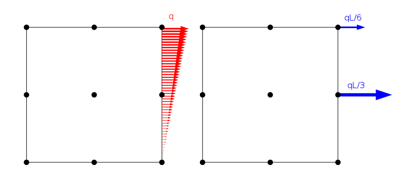
A linearly distributed load and how it is applied at the nodes of a second-order Lagrange element with side length L.
There is, however, an infinite number of load distributions that give the same nodal loads as long as they share the same resultant force and moment. Obviously, the solution to the finite element problem is the same for all of these cases. From Saint-Venant’s principle, however, we can conclude that all such loads should give essentially the same stress field as soon as we are some distance away.
Since the size of the area over which we redistribute loads is an element face, the linear dimension after which there is no difference is essentially one element layer inside the structure. Thus, the solution in the outermost layer of elements may not correspond to the actual load, but further in, it does.
As an example, we can load a rectangular plate with a boundary load that has an exponential stress distribution. The stress computed with a fine mesh is shown below.
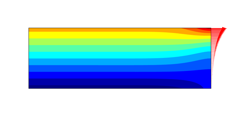
Contour plot of the axial stress distribution.
Because of Saint-Venant’s principle, the stress field is redistributed to a pure bending state at some distance from the loaded edge, just as we expect. This, however, is not the target of the current discussion. Rather, we investigate the difference between the stress distribution above, and what we get with a number of coarse meshes.
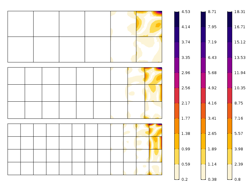
Error in axial stress for three different meshes. Note the different scales. As expected, the error is smaller when the mesh is finer.
As can be seen in the figure, the error quickly decreases after the first element layer. What we see here is actually a combination of mesh convergence and the redistribution of stresses implied by Saint-Venant’s principle.
Nonconforming Mesh
A nonconforming mesh occurs when the shape functions in two connected elements do not match. The most common case is when an assembly is connected using identity pairs and continuity conditions. To exemplify this, we can study a straight bar with an intentionally nonmatching mesh. With a simple load case, such as uniaxial tension, it is possible to study the stress disturbances caused by the transition.
Axial stress at a nonconforming mesh transition. Second-order elements are used.
The forces transmitted by the nodes at the two sides do not match the assumption of constant stress. Again, this can be seen as a local load redistribution over an area that is the element size. Using the reasoning of Saint-Venant, the disturbance should fade away at an “element-sized” distance from the transition. Let’s investigate what happens if the mesh is refined in the axial direction.
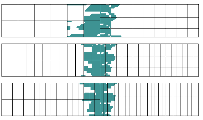
Region with more than 0.1% error in stress. Three different discretizations are used in the axial direction.
It turns out that the region of disturbance is not affected much by the discretization in the direction perpendicular to the transition boundary. This is exactly what Saint-Venant’s principle tells us.
Final Remarks
Without making use of Saint-Venant’s principle, many structural analyses are difficult to perform, simply because the detailed load distribution is not known.
The principle is formally only valid for linear elastic materials. In practice, we also intuitively use it on a daily basis for other situations. If, for example, the material in the “plate with a hole” example were elastoplastic, we would expect the two distributed loads to give equivalent results, as long as the yield stress is above the stress applied at the boundary so that there is only plastic deformation around the hole. The point load, however, always gives a different solution, since the material yields around the loaded point. For a longer discussion, read this blog post on singularities at point loads.
Next Steps
Learn more about using the COMSOL Multiphysics® software for FEA.
Further Reading
- Y.C. Fung and P. Tong, Classical and Computational Solid Mechanics, World Scientific Publishing Co. Pte. Ltd., 2001.


Comments (0)