
While reverse electrodialysis (RED) is a promising source of renewable energy, it can be a challenging process to analyze. The performance of RED units is affected by the physical phenomena that occur when converting salinity gradient energy into electric current. To address this, one team of researchers used a novel approach to model such systems in the COMSOL Multiphysics® software. Their multiphysics model and subsequent simulation studies provide further insight into designing and optimizing RED units.
Salinity Gradient as a Renewable Resource
Now more than ever, renewable energy sources like solar power and biofuels are helping to meet the world’s energy needs. According to the International Energy Agency, nearly 13.2% of the world’s energy consumption in 2012 came from renewable energy sources. Further, in 2013, about 22% of the energy used for global electricity generation was derived from renewable resources — a percentage that could increase by another 4% as of 2020. This growing demand fosters the need to identify more sources of renewable energy as well as optimize methods for obtaining it.

Biofuels (left) and solar power (right) are two sources of renewable energy. Left: Image by Idaho National Laboratory. Licensed under CC BY 2.0, via Flickr Creative Commons. Right: Image by minoru karamatsu. Licensed under CC BY 2.0, via Flickr Creative Commons.
One such energy source that has shown potential is salinity gradients. Salinity gradient power, also called osmotic power, refers to energy extracted through osmosis. This is the energy that causes water to spontaneously flow across a selectively permeable membrane, equalizing the concentrations of solutions on either side. Due to naturally occurring processes, saltwater and freshwater are salt solutions with different salt concentrations, meaning that salinity gradient power can be generated from readily available renewable sources. Salinity gradient power has the added benefit of releasing zero CO2 emissions. It also doesn’t produce toxic or contaminating waste, only brackish water.
But how do we harness this power? One method, which we will discuss here, is reverse electrodialysis.
Reverse Electrodialysis Harnesses the Power of Salinity Gradient
In osmosis, water moves across a selectively permeable membrane. An alternative way to extract the same energy is to use ion-exchange membranes, which are impermeable to water, but allow ions to move. Reverse electrodialysis (RED) are salinity gradient energy extraction systems that use ion-exchange membranes.
To understand RED, think of it as creating a salt battery. Freshwater and saltwater solutions pass through a stack of cells, which alternate between ion-exchange membranes (cation selective and anion selective). The concentration difference between the two solutions causes a voltage across each membrane, due to the driving force that equalizes the concentrations. Just as batteries can be linked in series to combine their voltages, the sum of the individual membrane voltages in a stack of cells gives the total voltage available from the RED system.
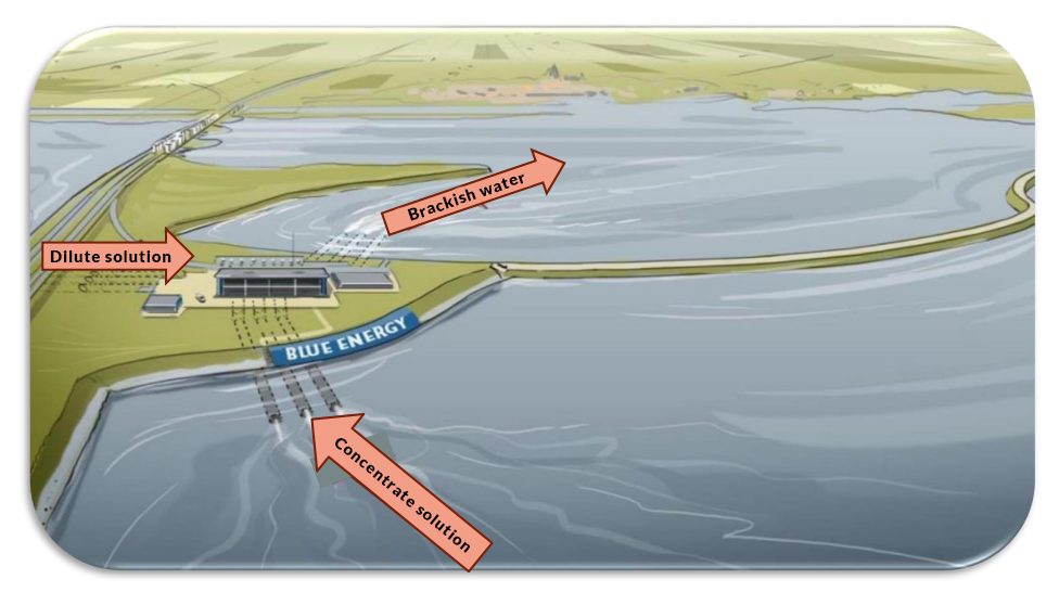
The RED process. Image by G. Battaglia, L. Gurreri, F. Santoro, A. Cipollina, A. Tamburini, G. Micale, and M. Ciofalo and taken from their COMSOL Conference 2016 Munich presentation.
The RED process includes multiple physics, from fluid dynamics to electrochemical transport phenomena. Analyzing this process can be difficult, as it requires a tool with the features and functionality to combine these different elements. To meet this challenge, a group of researchers from the University of Palermo in Italy turned to COMSOL Multiphysics, using a novel approach to model the RED process.
Designing a Multiphysics Model to Analyze Reverse Electrodialysis Units
For their analysis, the researchers created a 2D model of a single unit cell (cell pair) in the stack, composed of:
- Two half-anion exchange membranes (AEMs), since the unit cell is divided in the middle of the anion exchange membrane
- A concentrate flow compartment
- A cation exchange membrane (CEM)
- A dilute flow compartment
The schematic below shows the configuration of the cell pair, with each of the respective measurements included. Note that a cell pair section length of 1.2 mm was used to limit the computational load.
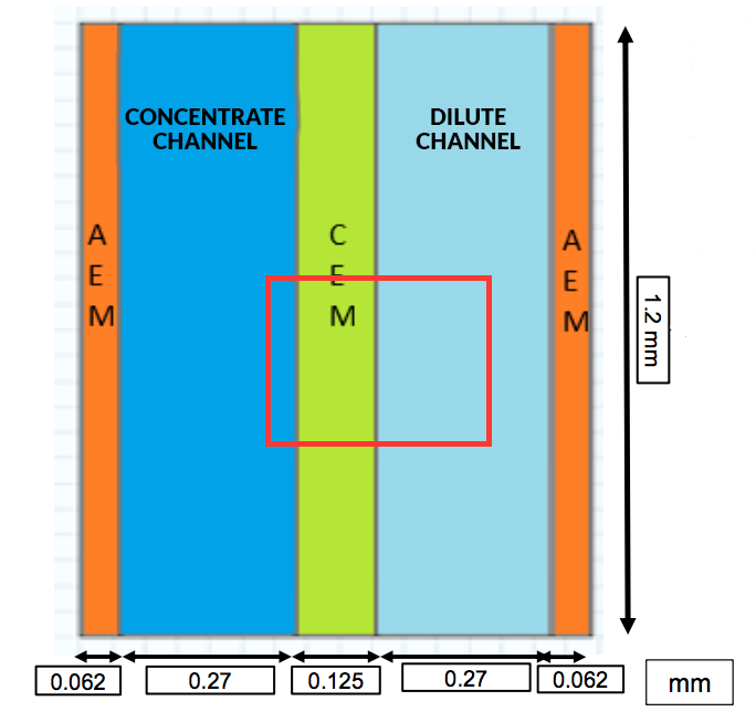
The computational domain. Image by G. Battaglia, L. Gurreri, F. Santoro, A. Cipollina, A. Tamburini, G. Micale, and M. Ciofalo and taken from their COMSOL Conference 2016 Munich presentation.
The researchers set the inlet velocities between 0.3 and 5 cm/s and the outlet pressures as 1 atm. For the inlet concentrations, they defined both channels to contain a solution of sodium chloride (NaCl). The concentrate channel was set as 4 M NaCl, while the dilute channel ranged between 0.005 and 0.5 M NaCl. These concentrations provide ideal conditions for power output, making use of concentrated brines (e.g., salty lakes) or in closed loops that regenerate concentrated solutions through evaporation from a low-grade heat between 50ºC and 100ºC (for instance, using solar energy).
The membranes were modeled as homogeneous and isotropic electrolytes with no fluid flow. Note that since few direct measurements were available, the researchers used experimental data to obtain ionic diffusivities and mobilities for the membranes. They also used experimental data to define the concentration of the fixed charges in the membranes. To account for the voltage losses at the interface between the ions and concentrate compartment, the researchers added a user-defined Donnan equation, which describes the contribution of membrane potential in the double layer.
Four different cell configurations were used in the analysis to evaluate typical channel designs. Often, these may include spacers for structural reasons. The configurations were:
- Empty channel
- Nonconductive round spacers
- Nonconductive square spacers
- Profiled membranes
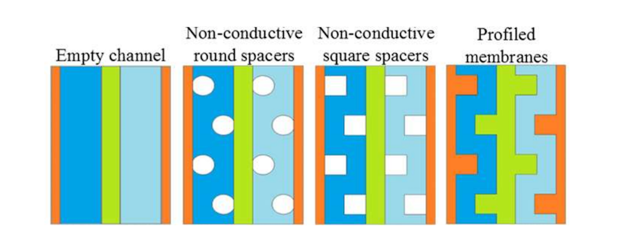
The different types of cell geometries used in the study. Note that the first three include a flat membrane. Image by G. Battaglia, L. Gurreri, F. Santoro, A. Cipollina, A. Tamburini, G. Micale, and M. Ciofalo and taken from their COMSOL Conference 2016 Munich paper.
Evaluating the Simulation Results in COMSOL Multiphysics®
All of the simulations were performed at a temperature of 20ºC under steady-state conditions. The solution steps were as follows:
- Solve the fluid dynamics of the system
- Solve for the electrochemical transport occurring within the system
- Solve for both physics together, using the previous solutions as inputs
Fluid Dynamics
Let’s begin by looking at the velocity map plot for the different geometric configurations, where an inlet velocity of 1 cm/s is used. Compared to the empty channel, the presence of obstacles causes the flow to change direction through the cell to locally accelerate the flow velocity and increase mass transfer to the membrane surfaces. With the profiled membranes, there is more contact area to the ion exchange membranes. However, there will also be more drag, as for the channels with obstacles, so a greater pressure drop is expected.
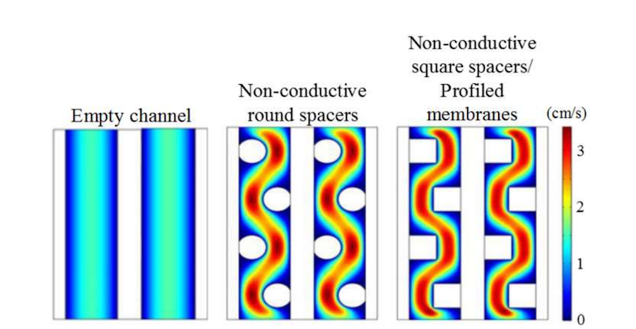
Velocity map plots for different geometric configurations. Image by G. Battaglia, L. Gurreri, F. Santoro, A. Cipollina, A. Tamburini, G. Micale, and M. Ciofalo and taken from their COMSOL Conference 2016 Munich paper.
Electrochemical Transport Phenomena
The next plot depicts the concentration profiles for a cell pair with an empty channel. Here, the membrane is fed by solutions of 0.5 M and 4 M, respectively, at 1 cm/s. In the solution, concentrations of sodium ions (Na+) and chloride ions (CI–) are equal to satisfy overall electroneutrality. However, in the membrane, they differ by a quantity that is equal to the concentrations of the fixed charges.
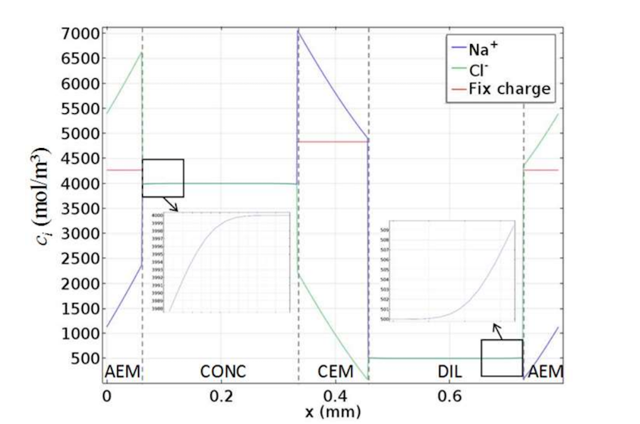
The concentration profiles for the cell pair with empty channels. Image by G. Battaglia, L. Gurreri, F. Santoro, A. Cipollina, A. Tamburini, G. Micale, and M. Ciofalo and taken from their COMSOL Conference 2016 Munich paper.
The following plot shows the membrane potential profiles at various external loads. At open circuit, the cell shows the maximum voltage (largest difference in potential from right to left). Looking at the results above, we see the concentration polarization phenomena inside the fluid domains where diffusion occurs due to the concentration differences, which lead to a voltage over the cell. No voltage losses occur because no electric current circulates.
On the other hand, losses occur when the circuit is closed. In this case, current is drawn through the stack and is carried through the solution and membrane by the ions. A diffusive flux in the boundary layer of the solution near the membrane ensures a balance of the electric field, but also introduces diffusional losses that reduce the membrane potential. These losses are greatest in the case of a short circuit (“short cut”), when the voltage over the cell would be zero.
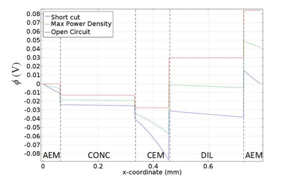
The potential profile for the cell pair with empty channels for different circuit conditions. Image by G. Battaglia, L. Gurreri, F. Santoro, A. Cipollina, A. Tamburini, G. Micale, and M. Ciofalo and taken from their COMSOL Conference 2016 Munich paper.
From the above plot, we can also see a significant voltage drop from Ohmic resistance within the membranes and, less notably, the 0.5 M dilute solution. The voltage drop is greatest in the membranes because they have lower electrical conductivity than the salt solutions. In contrast, the voltage drop is negligible in the highly conductive 4 M concentrate solution.
Another interesting observation is the effect of conductivity on the current density profile in more complex geometries, such as the case with profiled membranes. Current density likes to take the path of least resistance, which is basically through the more conductive concentrate solution, between membrane profiles, rather than through the membrane, leading to underutilization of parts of the cell. This becomes more pronounced when the concentration and conductivity in the dilute solution increases.
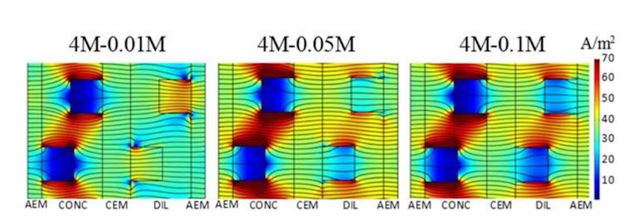
The current density distribution for the cell pair with profiled membranes. Compare the dense current density streamlines in the membranes on the left (lower-conductivity solution) with the lower membrane current density on the right (higher-conductivity solution). Image by G. Battaglia, L. Gurreri, F. Santoro, A. Cipollina, A. Tamburini, G. Micale, and M. Ciofalo and taken from their COMSOL Conference 2016 Munich paper.
Sensitivity Analysis
Next, let’s look at the results from a sensitivity analysis to see how the membrane/channel configuration, dilute concentration, and feed velocity impact the net power density. The plot below depicts the overall resistance of the cell pair for different dilute concentrations and membrane/channel configurations.
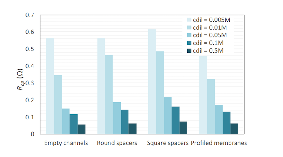
The cell pair resistance for various dilute concentrations and membrane/channel configurations. Image by G. Battaglia, L. Gurreri, F. Santoro, A. Cipollina, A. Tamburini, G. Micale, and M. Ciofalo and taken from their COMSOL Conference 2016 Munich paper.
As the results show, the cell pair resistance decreases as the dilute concentration increases. This can be attributed to the higher conductivity of these solutions. The lowest resistance is given by the empty channel configuration at higher concentrations, while the highest resistance is given by the nonconductive spacers in all cases. Only when a dilute concentrate is less than or equal to 0.01 M is a profiled membrane effective; empty channels perform better in more conductive solutions.
In the plot below, we see the net power densities for different configurations and dilute concentrations. This considers both the power density delivered by the cell and the power costs to pump the flow, thus the costs that impeding the flow add to the process. The profiled membrane achieves the highest net power density at about 4.4 W/m2 for a dilute solution of 0.01 M. Configurations with spacers (especially square ones) have greater flow resistance and pressure drop, resulting in lower net power densities. For dilute concentrations less than or equal to 0.01 M, profiled membranes improve process performance with respect to empty channels.
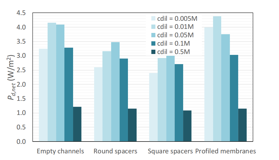
The maximum net power density for various dilute concentrations and membrane/channel configurations. Image by G. Battaglia, L. Gurreri, F. Santoro, A. Cipollina, A. Tamburini, G. Micale, and M. Ciofalo and taken from their COMSOL Conference 2016 Munich paper.
By showing the power density as a function of the configuration, the above results help designers to identify the optimal components, geometry, and conditions for their channel. Without the use of simulation, such conclusions are not necessarily so obvious.
Simulation Helps Advance the Design and Performance of RED Units
For the RED process to become a more efficient means of obtaining renewable energy, it is important that we have tools to perform complex analyses with accuracy. As the research presented here shows, COMSOL Multiphysics is a tool that meets this challenge by providing comprehensive features and functionality to address multiphysics problems.
Learn More About Using Simulation to Study Renewable Energy
- Read the full COMSOL Conference 2016 paper: “Investigation of Reverse ElectroDialysis Units by Multi-Physical Modelling“
- See other uses of simulation to advance renewable energy processes:


Comments (0)