Using Lumped Ports and Lumped Elements in Electromagnetic Field Modeling
When modeling frequency-domain and time-domain electromagnetic fields in the Magnetic Fields interface in the AC/DC Module, an add-on to the COMSOL Multiphysics® software, the Lumped Port boundary condition can be used to model a connection to a source or to an arbitrary electrical load. The Lumped Element node is similar to the Lumped Port boundary condition and represents loads of certain types.
Both features have four geometry types that affect the shape of the boundary at which it can applied. The Lumped Port boundary condition has three different terminal types that affect how the connected source or load is modeled. This guide goes through these geometry- and terminal-type options for frequency-domain and time-domain modeling.
The Excitation and Load Options for Frequency-Domain Modeling
The Lumped Port boundary condition represents the terminal of a transmission line (a cable) connected to the modeling space. The three options for Terminal types are Current, Cable, and Circuit, and these can be combined within a single model. The Lumped Element node represents a connection to a lumped impedance that can be complex-valued.
The Current type imposes a specified current,  , going through the model and induces electric and magnetic fields throughout the modeled space. If there are multiple Lumped Port conditions of type Current, then a complex-valued imposed current is equivalent to a phase shift between them. For example, imposed currents of ,
  , and
, and  at three different lumped ports correspond to three-phase excitation. For more details on working with complex-valued numbers in the frequency domain, see our article on this topic.
The induced electric fields at the Lumped Port boundary condition are integrated to compute the port voltage,  . This port voltage is complex-valued, and if it is the only source in the model, it is used to compute the port impedance,
  , as well as the cycle-averaged power,
  , delivered to the model. It is also possible to impose zero current, which represents an open-circuit configuration. In this situation, the only output is the open-circuit voltage at that terminal induced by all other sources in the model.
The Cable type is similar to the Current type and includes a parallel resistor of specified characteristic impedance,  . This impedance represents a transmission line, so even when there is no excitation, the Cable type represents a real-valued impedance connected to the system. For the Cable type, the excitation is explicitly specified as On or Off. When the excitation is On, the Source type option can be set as either Voltage or Power. Both of these options impose a current based on the assumption that the impedance of the modeled system matches the cable impedance. That is, the total impedance seen by the current source is assumed to be half the cable impedance. So, when Voltage,
  , is specified, then the imposed current is
  , and a phase shift between excited lumped ports can be introduced via a complex-valued voltage or a nonzero Port Phase. When Power,
  , is specified, then the imposed current is
  .
.
For the Cable type, the computed port current,  , is the current going through the model, and the port voltage, , will be different from the specified voltage, , unless the impedance of the model exactly matches the cable impedance. The computed port impedance is
  . For a model with one or more Lumped Port boundary condition of terminal type Cable, the S-parameters will also be computed.
The Circuit type represents a connection to an arbitrary combination of lumped electrical elements, including resistors, capacitors, inductors, mutual inductance, and transformers as well as current and voltage sources. This combination can be of arbitrary complexity, but all lumped electrical elements in a frequency-domain model must be linear, so elements like diodes and switches instead need to be addressed via a time-domain model.
The Lumped Element node represents a connection to an arbitrary impedance. The impedance is defined as a combination of a resistor, capacitor, and inductor in series or in parallel or a user-defined impedance, which allows for an arbitrary complex-valued impedance as a function of frequency.
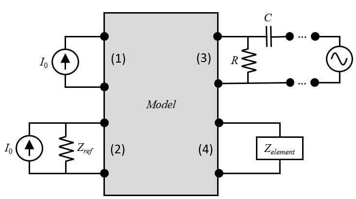
The Lumped Port boundary condition can be of type Current (1), Cable (2), or Circuit (3) and can represent excited or unexcited connections, whereas the Lumped Element node (4) solely represents an impedance; it does not include any excitation.
Geometry Types
Both the Lumped Port and the Lumped Element feature have multiple geometry-type options: Via, User Defined, Uniform, and Coaxial. These affect the shape and topology of the boundaries at which they can be applied.
Via
The Via type is meant to be used along a straight section of a circular conductor — a wire. It has to be applied on a set of faces that describe the complete circular perimeter of the wire. This boundary condition imposes a uniform current density around its entire perimeter, flowing parallel to its axis. The cylindrical domain inside of the lumped port should be omitted from the model. Although the Via type can be placed anywhere along the length of a wire, its most accurate usage is in a region of the model where the fields can be expected to be nearly invariant in the axial and azimuthal directions. It can also be used on a set of cylindrical faces placed between noncylindrical conductive domains or conductive boundaries.
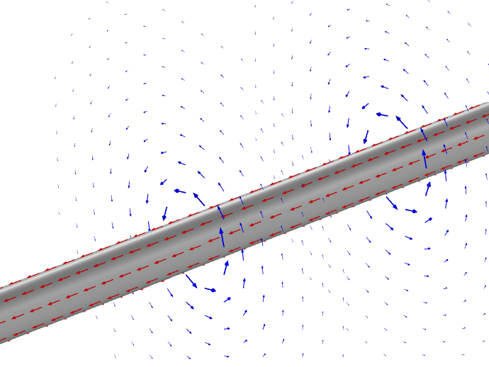 A gray wire with red arrows along the wire and blue arrows pointing in a counterclockwise direction around the wire.
Current (red arrows) flowing along a straight section of wire and the surrounding magnetic field (blue arrows). The fields are invariant in the azimuthal direction and along the length.
When the volume of the adjacent conductor is being modeled, the cross-sectional faces at either end of the lumped port should be set to Magnetic Insulation, implying an equipotential condition over the cross section. The imposed current flowing along the lumped port boundary will induce currents in the adjacent domains and boundaries.
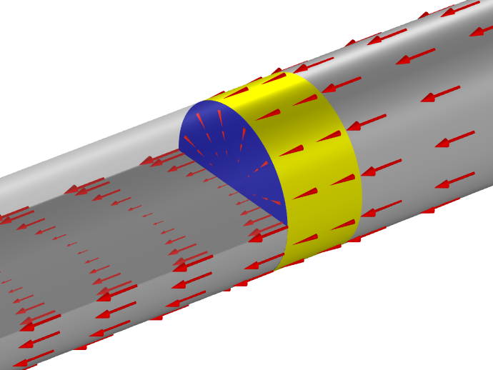 A gray wire with a half transparent blue boundary and red cones and arrows showing the current direction.
A Via-type Lumped Port boundary condition is applied at the yellow surfaces that bridge a gap along the circular wire. The imposed lumped port current induces surface currents (red cones) on the magnetic insulation boundaries (blue) that are at the cross sections of the conductors. Volumetric currents (red arrows) that exhibit the skin effect are induced within the volume of the conductive domains (gray).
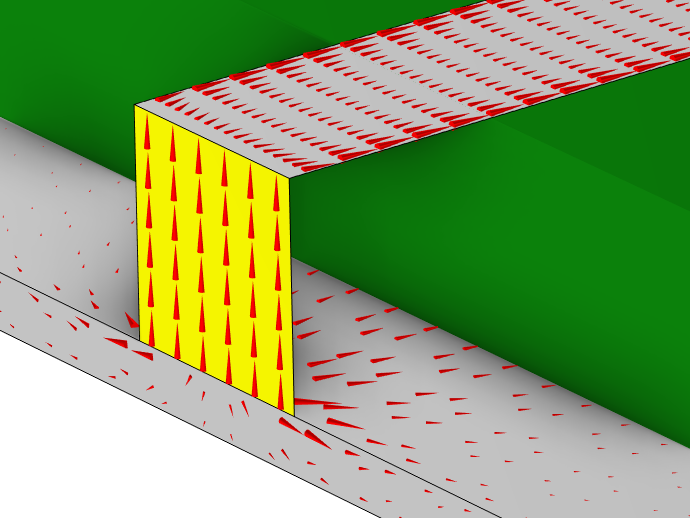
The Via type is also meant to be used between the layers of metallization of a circuit board. In this situation, one or both of the adjacent conductors may be modeled as conductive boundary conditions of zero geometric thickness.
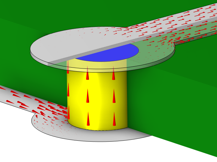 A yellow semicylinder connected to a green circuit board with gray connectors and red arrows showing the excitation direction.
A Via-type Lumped Port boundary condition excitation between two conductive traces of a circuit board. The traces can be modeled either as boundary conditions or as volumes.
Uniform
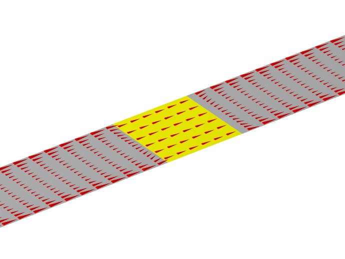
The Uniform type can only be applied to a rectangular face that bridges a gap between a combination of either Magnetic Insulation, Impedance, or Transition boundary conditions. The imposed surface current is in the direction between these conductive boundaries. The Uniform type is reasonable to use for exciting a microstrip, either along its length or relative to a ground plane, or for introducing a Lumped Element impedance between conductors. Since the Uniform type exists entirely within the volume of the modeled space, it excites fields on both sides. The source, and load, can be thought of as existing on the surface itself without occupying any volume. It is a more approximate condition and can be substituted with a Via type if higher accuracy is desired.
 A gray rectangle highlighting a yellow section with red cones to show the surface current.
A Uniform-type Lumped Port boundary condition excitation (yellow) along the length of a conductive strip (gray) modeled as a Transition Boundary Condition. The surface currents (red cones) are uniform across the lumped port, but on the conductive surface, inductive effects drive the currents toward the edges.
 A yellow uniform lumped port above a ground plane with red cones showing the excitation current of a stripline.
A Uniform-type Lumped Port boundary condition used to excite a stripline above a ground plane.
 A blue and yellow lumped element model between two gray wires with red cones to show the current.
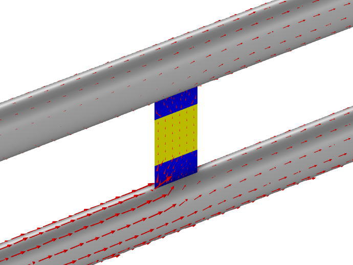
A Uniform-type Lumped Element node placed between two Magnetic Insulation boundary conditions is used to introduce an impedance between two conductive wires. The current flowing within the volume of the wire flows onto the Magnetic Insulation and Lumped Element boundaries.
User Defined
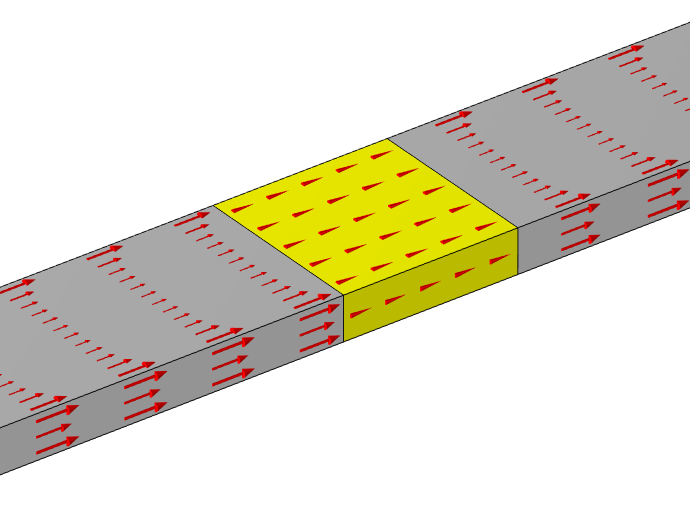
The User Defined type is primarily useful for connections to noncircular wires. The direction, height, and width of the lumped port needs to be entered manually. These correspond to the direction in which the current is being driven; the distance across the lumped port; and the width, or perimeter, of the set of selected faces.
 A gray rectangular prism highlighting a yellow user-defined section with red cones and arrows.
A User Defined-type Lumped Port boundary condition placed along a noncircular wire. The user-defined direction is a vector between the conductors, the height is the distance between them, and the width is the perimeter of the conductor.
Coaxial
The Coaxial type is applied to an annular face that describes a cross section through the dielectric domain between the inner and outer conductor of a coaxial cable. The inner and outer conductors can be modeled either as solid conductors, as Magnetic Insulation boundary conditions, or as the Impedance Boundary Condition. The coaxial lumped port imposes a current along the surface that matches the analytic displacement currents within a lossless cable, so if the inner and outer conductors are modeled using Magnetic Insulation boundary conditions, then the fields next to the Coaxial-type Lumped Port boundary condition will approach the exact analytic solution, in the limit of mesh refinement.
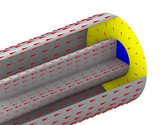 A transparent gray tube with a blue magnetic insulation boundary condition showing red cones and arrows to represent the excitation.
The Coaxial-type Lumped Port condition has to be applied to an annular face (yellow) between an inner and outer conductor (gray) that can be modeled as a boundary condition or as a volume. If the conductor is modeled as a volume, then the Magnetic Insulation boundary condition (blue) must be adjacent to the Lumped Port boundary condition.
The Excitation and Load Options for Time-Domain Modeling
When modeling in the time domain, there are a few differences in the excitations and loads. The Current type excitation can accept any time-varying expression. The Cable type excitation can only accept a Voltage excitation. When evaluating outputs (voltage, current, power, impedance), these are all instantaneous quantities.
The Circuit type allows for a connection to a system consisting of any arbitrary lumped electrical elements, including those with nonlinear response.
The Lumped Element feature admits only real-valued impedance; it cannot be used to add inductive or capacitive loads in a time-domain model.
The Transition Boundary Condition and Impedance Boundary Condition features are not available for time-domain modeling. All lossy materials need to be modeled as domains.
Submit feedback about this page or contact support here.