Learning Center

Understanding the Options for Meshing and Geometric Modeling of Conductors in Electromagnetic Fields

---

This guide addresses the meshing and geometric modeling of conductors exposed to steady-state, arbitrarily-time-varying, or sinusoidally varying electromagnetic fields. These conditions require that the model considers the distribution of current over the cross section of the conductor to accurately model the fields and losses. The magnetic fields can arise either due to an external source or to currents being driven through the conductor. 

Background: The Skin Effect

Whenever a lossy material is exposed to a time-varying electromagnetic field, there will be induced currents, and these act to cancel any currents flowing within the interior of the material. For a material with electric conductivity , relative permittivity , and relative permeability , exposed to a sinusoidally varying signal of angular frequency , it is possible to define a skin depth:

This is the distance into the volume over which the current decreases in magnitude by compared to the current at the surface. A simpler expression can be used for metals:

These different regimes, where the skin depth is either large, comparable, or small compared to the dimensions of the conductor, each motivate a set of different meshing and geometric modeling techniques. These techniques are presented in terms of computing the losses within the conductor. Losses are proportional to the square of the current , so monitoring convergence of losses with respect to mesh refinement is motivated.

The Testcase Model 

The meshing and modeling of the conductor will be studied in the context of a rounded square loop of copper wire. The wire has a radius of 1 mm, the square loop has a width of 4 mm, and the bends have a radius of 2 mm. This loop is placed within the center of a long multiturn solenoid composed of wires that are assumed to be exactly parallel, so the current is assumed to flow only in the azimuthal direction. 

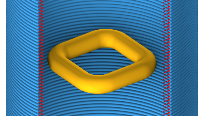
A square loop of copper wire, with rounded corners, inside of a long solenoid.

Symmetry can be exploited to reduce the model to a 45^° section of the loop, and mirrored about its plane. The Magnetic Insulation boundary condition in COMSOL Multiphysics^® imposes symmetry on the sides. The Perfect Magnetic Conductor boundary condition is used on the bottom and top boundaries implying an infinite array of these wire loops extending along the axis. The solenoid can be modeled as a surface current flowing in the azimuthal direction, and the space outside of the solenoid does not need to be modeled. 

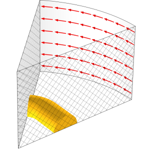
Visualization of the modeling domain. Symmetry is imposed by the Magnetic Insulation boundary conditions (crosshatched) and the Perfect Magnetic Condition (top and bottom, transparent). The Surface Current Density condition imposes a sinusoidally varying current flow in the azimuthal direction (red arrows), and this imposes currents into the loop of copper wire.

The mesh is shown with an element size in the wire such that there are 32 elements around the entire perimeter (16 elements about the half) and element size equal to radius in the surrounding space.

The element size within the wire is selected based on the wire perimeter (2pir) starting with an element size that is one-eighth of the perimeter, and the model is rerun with a size of 1/16 and 1/32 of the perimeter, with the finest mesh shown below.

The model is solved over the frequency range of 60 Hz–60 MHz, corresponding to a skin depth of 8.4 mm–8.4 µm, or approximately 10 times greater than the radius, to approximately 100 times smaller than the radius. The model is meshed with a global maximum element size of 1 mm, and with different meshing and geometric modeling strategies within the wire.

The Low-Frequency Range

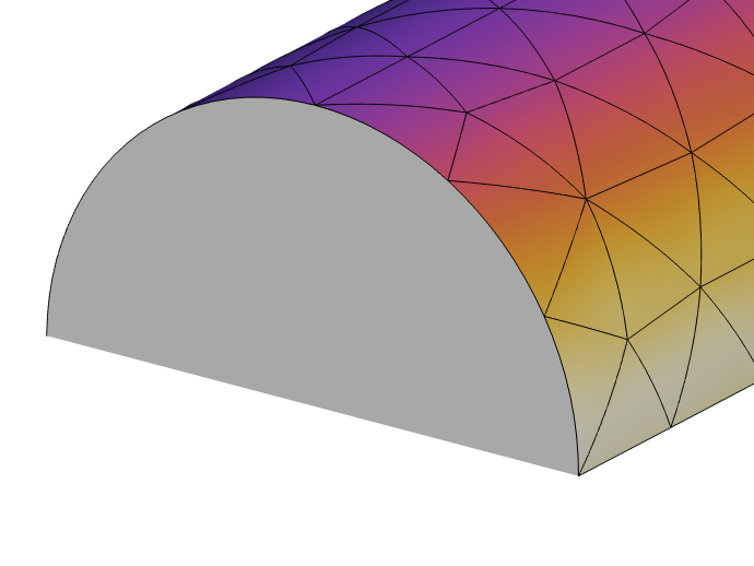
In this regime, it is only necessary to refine the mesh sufficiently to give good resolution of the geometry. To demonstrate, the element size within the wire is selected based on the wire perimeter, starting with an element size that is one-eighth of the perimeter, and the model is rerun with a size of 1/16 and 1/32 of the perimeter, with the finest mesh shown below.

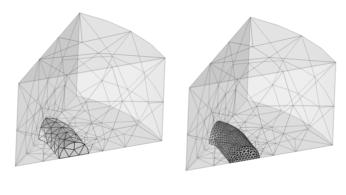
Visualization of the mesh, with an element size in the wire of 1/8 and 1/32 of the perimeter. The element size in the surrounding space can be much larger.

These types of modifications to the mesh are done by setting up a user-defined mesh, with a set of Size features.

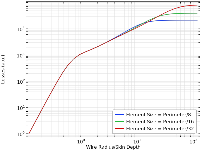
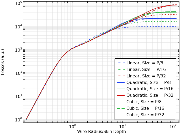
The plot below shows the losses over the 60 Hz–60 MHz frequency range. The horizontal axis of the plot is presented in terms of the radius of the wire divided by the skin depth of the material. It is more general to discuss these results in terms of the characteristic dimension normalized with respect to skin depth, rather than frequency. When the wire radius is much smaller than the skin depth, the solution is almost identical between all meshes. Once the skin depth starts becoming smaller than the radius, deviations between the meshes appear. The losses are about 20% different between the different meshes once the skin depth in one-tenth of the radius, and the deviations increase even more with increasing frequency (smaller skin depth) beyond that point. 

A 1D plot with losses on the y-axis and wire radius/skin depth on the x-axis.

Plot of the losses (in arbitrary units) versus frequency normalized in terms of skin depth and wire radius. Good agreement is observed over a wide frequency range, but results diverge and become less accurate at higher frequencies.

This plot is repeated for first-order and third-order discretization, the linear and quadratic elements, showing very similar results up to the point where skin depth equals radius. At higher frequencies we can see that linear elements do lead to slightly different results, and conductors should be meshed more finely. 

A 1D plot with losses on the y-axis and wire radius/skin depth on the x-axis.

Comparison of computed losses with different mesh sizes and element order. High-order elements are more accurate.

These plots give a definition of the low-frequency range: The mesh need only be sufficiently fine to resolve the geometry. A useful rule of thumb for meshing of geometry is that 90^° arcs need to be meshed with at least two elements when using quadratic or higher discretization, and more than four elements if using linear discretization. Or: The perimeter of a circular wire should be meshed with at least eight elements when using the quadratic or cubic discretization, or more than 16 elements when using linear discretization.

It is generally recommended to use the default quadratic discretization; higher discretization will use significantly more memory for only small improvements in accuracy. Linear discretization is primarily motivated when solving models that also include a material nonlinearity, such as a nonlinear B-H curve. The remainder of this article focuses on using quadratic discretization.

The Intermediate Frequency Range

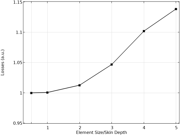
It is useful as a first step to focus on one point in the frequency range, the frequency at which the wire radius is ten times larger than the skin depth, and to study losses with even further mesh refinement. Rather than defining the mesh size in terms of the geometric dimensions, the element size is defined as a multiple of the skin depth. The figure below shows the losses as the mesh is refined, normalized with respect to the losses at the peak level of refinement. This plot shows the expected convergence behavior; as the mesh is refined, a more accurate solution at this frequency is obtained. It is also reasonable to infer that having an element size equal to the skin depth, or smaller, will accurately compute the losses. 

A 1D plot with a black line and six points with losses on the y-axis and element size/skin depth on the x-axis.

Mesh convergence study at a single frequency, where the wire radius is ten times larger than the skin depth. As element size decreases below the skin depth, the integral of the losses over the wire changes minimally.

Such a fine mesh is, in general, going to be impractical. The figure below shows the distribution of the losses within the wire, and as expected, these are very close to the surface. The fine mesh deeper within the interior of the wire does not provide much benefit in terms of accuracy and greatly increases the computational cost. 

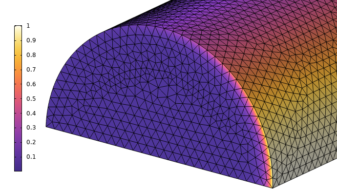
The distribution of the losses within the wire, at a frequency where the skin depth is one-tenth of the radius.

It is thus desirable to find a meshing strategy that gives good resolution of the significant variation in the losses in the direction normal to the boundary, and this is achieved via a Boundary Layer Mesh feature. This feature introduces several thin layers of elements normal to the boundary, as visualized below. The thickness of the first layer can be selected to be about equal to the skin depth at the highest frequency, and each subsequent layer can be 1.5–2.5 times thicker than the previous, until the total thickness of the boundary layer elements is about one-tenth of the radius. 

The boundary layer mesh combines a good resolution of the fields tangential and normal to the boundary of the conductor.

The High-Frequency Range

Once the cross-sectional dimensions of the conductor become significantly larger that the skin depth, it becomes increasingly less necessary to model the interior volume of the conductor. In this range, the currents and losses within the volume are very close to the surface, and the interior is very well shielded. This regime is very well approximated by omitting the interior volume of the conductor from the model and using the Impedance Boundary Condition on the exterior surfaces of the coil. This feature, which is only applicable in a frequency-domain model, computes currents and losses on the surface of the domain due to the conductivity of the material within the domain. 

The Impedance Boundary Condition computes losses on the surface under the assumption that the skin depth is small compared to the conductor cross-sectional dimensions.

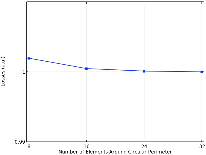
Within this range, it is only important for the mesh to accurately resolve the surface of the conductor, in terms of the geometric shape and the variation in the currents across the surface. Similarly to the low-frequency range, the losses are studied in terms of the number of elements around the perimeter of this circular wire. The results below show that a mesh with only eight elements around the perimeter of this circular wire, or two elements per 90^° arc, are very accurate. These results were generated at a frequency of 60 MHz, where the skin depth is 100 times smaller than the wire radius.

A 1D plot with a blue line and four points with losses on the y-axis and number of elements around circular perimeter on the x-axis.

Mesh convergence study when using Impedance Boundary Condition.

Combining Intermediate and High-Frequency Ranges

It can be useful to modify the geometry of the model to create a hybrid of the intermediate frequency and high-frequency range modeling techniques. This is done by partitioning the conductor into two regions, one thin layer at the boundary of the material, and a second region within that, which is not modeled, as illustrated below. The Impedance Boundary Condition can then be applied at the boundaries between these domains. This hybrid approach reduces computational cost by omitting the interior of the conductor yet gives high accuracy at low cost of the currents flowing primarily tangentially to the boundary.

Partitioning of the conductor into two domains, an outer layer within which the fields are solved for, and an inner domain, where the fields are not solved for. The Impedance Boundary Condition is applied at the boundary between these domains.

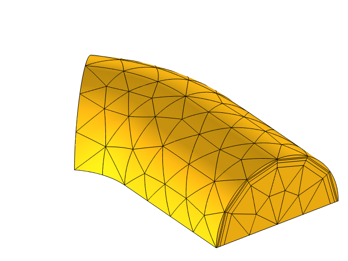
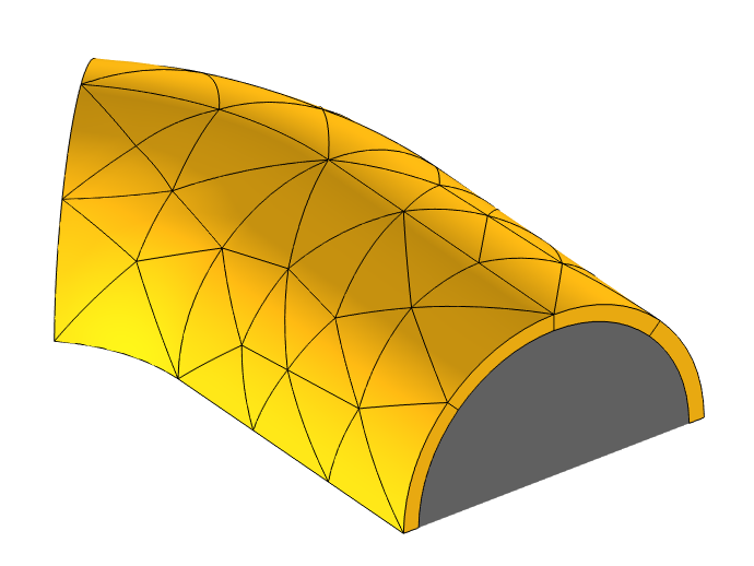
This hybrid approach requires choosing the layer thickness based on the operating frequency, and is only appropriate for solving at single, or a narrow band of, frequencies. It is possible to extend this approach by using multiple layers of different thicknesses, which allows for a much wider band of frequencies to be modeled. The volume of the interior, inside of the layers, can also be modeled. The thickness of the first layer should be equal to the smallest skin depth over the frequency range of interest, and the growth factor in the thickness should be between 1.5–3, with the number of layers adjusted such that the total thickness of the layers is one-tenth of the characteristic dimension of the conductor. A sample of such a mesh is shown below. Note that all domains of the conductor are modeled. 

Partitioning of the conductor with several layers along the outside that will resolve the losses over a wide band of frequencies. The entire volume of the conductor is modeled.

Comparison of Methods

The wideband approach, which introduces additional layers, can be used to set up a highly refined model that can be used as a basis of comparison of the other approaches. This comparison is presented below. Several conclusions can be made:

• If the skin depth is comparable to the cross-sectional dimension (in this case, the radius), then the low-frequency approach of using a tetrahedral mesh that resolves the geometry accurately is sufficient.
• Boundary layer meshing is appropriate until the skin depth approaches 100 times smaller than the radius. 
• If solving at a single frequency, the hybrid approach can be very efficient. 
• If the skin depth is very small, (~100x) compared to the radius, then using the impedance boundary condition instead of modeling the conductor is also appropriate. 

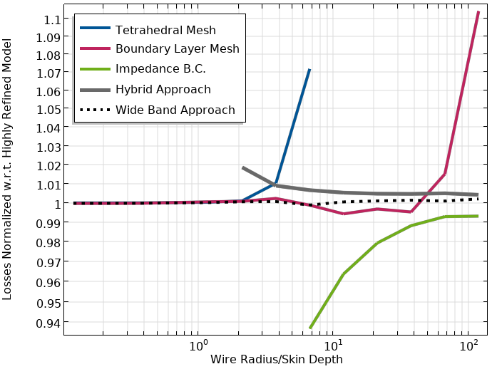A 1D plot with losses normalized on the y-axis and wire radius/skin depth on the x-axis.

Comparison of approaches over a wide frequency range. All solutions are normalized with respect to a solution computed with a highly refined mesh.

The various meshing techniques demonstrated in the companion file are meant to provide an overview of the meshing strategies for conductors that have smooth sides without sharp corners. Fundamentally, the mesh size needs to resolve the skin depth. If the skin depth becomes smaller than the cross section, then boundary layer meshing as well as partitioning of the geometry are computationally efficient approaches. If the skin depth is over one hundred times smaller than the cross-sectional dimensions, then using the impedance boundary condition becomes a good modeling approach.

Transient and DC Modeling

When solving a problem involving variation in time, it is important to fully understand the frequency content of the applied signals. This can be done by using the Fourier transform functionality, as described in our article "Understanding Periodic Signals and Their Frequency Content". Once the frequency content is known, either the wideband modeling approach or the boundary layer meshing approach should be used. The wideband model is better when the smallest skin depth of interest is much smaller than the dimensions. If solving a transient model where the excitation is single-frequency, then the hybrid approach can be useful. The Impedance Boundary Condition is not available for time-domain modeling; the Magnetic Insulation boundary condition can be used instead, which implies a perfectly conductive domain with all currents flowing on the surface. 

When solving DC problems, with no variation in time, the meshing strategy is identical to the low-frequency case. There will be no skin effect, so the solution within the conductor will usually be accurately computed as long as the mesh accurately represents the geometry.