Homogenization of Material Properties
In the COMSOL Multiphysics® software, there are several capabilities that enable you to perform homogenization of material properties. This includes using different physics interfaces, boundary conditions, and homogenization methods. Here, we outline how to implement material homogenization through these different techniques. Additionally, we highlight a simulation app that enables you to compute the homogenized properties of composite materials and show several relevant tutorial models.
Background
Continuum mechanics is based on the concept of homogeneous materials where the infinitesimal subvolume of the material possesses the same material properties as the bulk material. In reality, at some scale, all materials are heterogeneous. Monolithic material, which is made of a single constituent, is considered homogeneous at bulk as well as infinitesimal subvolume levels — ignoring any heterogeneity at, for example, the grain level. The materials made of two or more constituents, called composite materials, are heterogeneous at a micro level, and to be analyzed at a macro level they need to be treated as an effective or pseudohomogeneous continuum. Experimental methods can be used to find out the homogeneous or effective properties of composite materials. These methods are time- and cost-consuming, so alternative methods that are reliable and easy to use are needed. Homogenization methods are mathematical methods that provide alternatives to these experimental methods.
Homogenization methods find the effective, or homogeneous, material properties of composite materials based on their microstructure. Homogenization is the study of the relationship between a material microstructure and its macroscopic behavior. The scope of homogenization methods is not limited to the material microstructure but is also applicable to monolithic material with geometrical periodicity. In the case of corrugated or perforated sheets (geometric periodicity), homogenization methods can be used to find the effective properties so that they can be treated as the equivalent flat orthotropic sheets, which makes numerical analysis easier.
Based on the underlying formulation, the homogenization methods can be divided into two main classes:
- Analytical methods
- Numerical methods
In the field of structural mechanics, structures can be analyzed in different mathematical space dimensions depending on the geometry of the structure. Although numerical homogenization models in solids, shells, and beams are based on the same concept, the actual implementation differs based on the applied boundary conditions. In this article, we will explore homogenization in solids, shells, and beams separately.
Note that in the literature, homogeneous material properties are also known as effective properties, equivalent properties, and average properties. In this article, these words are used interchangeably.
Analytical Methods
There are several analytical models available for computing the effective material properties of solid, liquid, or gas mixtures. The analytical models are also called rule of mixtures. Some of them are explained below.
Model 1: Volume Average
This is an elementary model for a mixture with isotropic constituents where the effective properties are the arithmetic mean of constituent properties weighted by the volume fractions,

where  is the number of phases,
  is the volume fraction of constituent
  ,
,  is the material property of constituent , and
  is the effective property. This type of averaging is relevant for the mass density, for example. Similar to the volume average, other analytical models for mixtures with isotropic constituents are mass average, harmonic volume average, harmonic mass average, power law, and Heaviside function. All of these analytical models are available in the Multiphase Material node under Materials (pictured below).

The settings for a Multiphase Material node.
The multiphase material can be used with multiple phases with different volume fractions. This material can be used for solid, liquid, or gas mixtures alike. If we instead focus on the analytical models used for solid mixtures, i.e., composite materials, then the rule of mixtures are as follows:
Model 2: Voigt–Reuss
Most composites have direction-dependent material properties, so the analytical models must be direction dependent. One simple example of this type of model is the Voigt–Reuss model. This method works well when continuous orthotropic fibers are embedded in an isotropic matrix. The figures below show two kinds of unidirectional fiber composites.

Unidirectional fiber composite with square packing (left) and hexagonal packing (right).
The Young's moduli, Poisson's ratios, and shear moduli are given as:
| Material Property | Component | Effective Property |
|---|---|---|
Young's Moduli,  |
 |
 |
| Young's Moduli, |
 |
 |
| Young's Moduli, |
 |
 |
Shear Moduli,  |
 |
 |
| Shear Moduli, |
 |
 |
| Shear Moduli, |
 |
 |
Poisson's ratios,  |
 |
 |
| Poisson's ratios, |
 |
 |
| Poisson's ratios, |
 |
 |
These expressions allow more than two phases, but for an ordinary fiber composite where n = 2, one phase is the fiber material, and the other is the matrix. The fibers are oriented in the local 1-direction.
Similar to the Voigt–Reuss model, the Modified Voigt–Reuss, Chamis, Halpin–Tsai, Halpin–Tsi-Nielsen, and Hashin–Rosen models are available (shown below) and suitable for orthotropic composite materials.
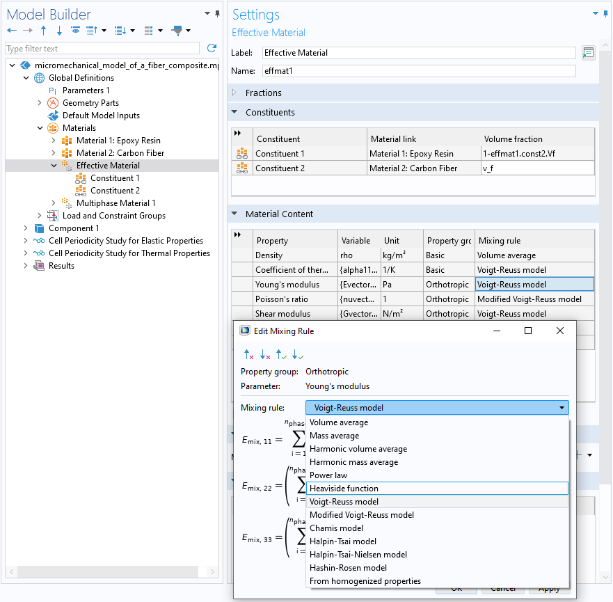
The settings for an Effective Material node.
The effective material is analogous to the multiphase material, but it has composite-specific analytical models in addition to the elementary models. These analytical models are mostly suited for composites made of two constituents, which caters to most real-life materials.
Numerical Methods
There are different numerical methods for the homogenization of composite materials. For example:
- Finite element homogenization
- Finite difference homogenization
- Boundary element homogenization
- Eshelby homogenization
- Mean field homogenization
In this article, we are focusing on the finite element homogenization. Representative volume elements (RVEs) or repeating unit cells (RUCs) of the heterogeneous material are used, and appropriate boundary conditions or tractions are applied to obtain the effective material properties. The scope of this presentation is limited to linear constitutive relations together with an assumption about geometric linearity. In some cases, it is possible to extend the homogenization techniques to include nonlinear cases, but that is more complicated. The basics of finite element homogenization are the same in all space dimensions or for all structural elements. The discussion is split into three distinct parts: homogenization in solids, homogenization in shells, and homogenization in beams.
Homogenization in Solids
Homogenization in solids requires the application of appropriate boundary conditions or tractions to the RVE or RUC. Before introducing the details of the mathematics, the difference between RVEs and RUCs must be discussed, as there can be a misconception that both concepts are the same, despite the fact that they differ in their fundamentals. An RVE is a subvolume that characterizes heterogeneous material with statically homogeneous microstructures at an appropriate scale. To get effective material properties with RVE, one needs to apply homogeneous displacement or traction boundary conditions. The RUC, or unit cell, is a material subvolume that characterizes periodic heterogeneous materials. The RUC is a material subvolume that can be repeated in all space directions to create a material at bulk level. An RUC needs periodic boundary conditions to get the effective material properties. In short, the RVE is a top-to-bottom approach where the boundary conditions are applied to the material subvolume just as they could have applied to the actual homogeneous material. The RUC is a bottom-to-top approach, as each subvolume of the material is identical and the material is truly periodic in nature. The RUC applies solely to materials with a genuinely periodic microstructure, whereas the RVE can be employed for microstructures that are either periodic or nonperiodic. However, the accuracy of homogenized material properties derived through the RVE approach for periodic materials depends on the size of the material subvolume. For more details, see References 1 and 2. The concepts of RVEs and RUCs are illustrated below.
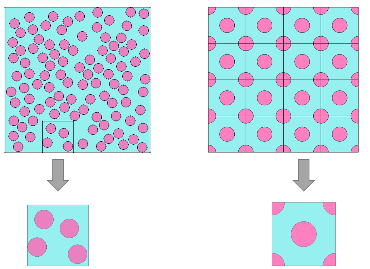 Two side-by-side microstructure figures, with the left microstructure characterized by an RVE (bottom left) and the microstructure on the right characterized by an RUC (bottom right).
A microscopically heterogeneous microstructure characterized by an RVE (left) and RUC (right).
In COMSOL Multiphysics®, parametric geometric parts are available to be used as RVEs or RUCs. You can find several such geometries in the Part Libraries.
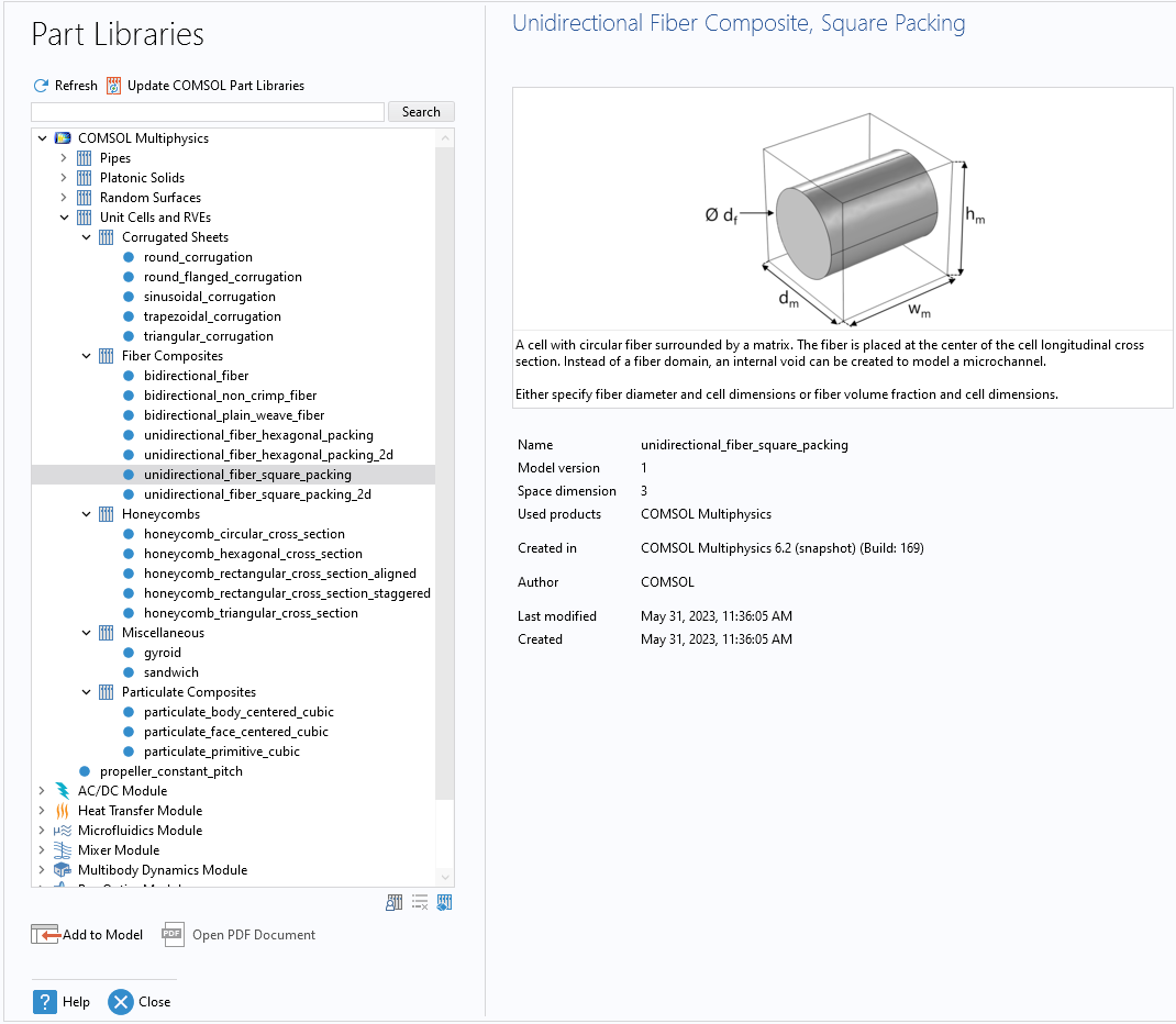 The Part Libraries with the Unidirectional Fiber Composite, Square Packing model selected.
The Part Libraries window with the geometry part tree for unit cells and RVEs expanded.
Periodic Boundary Condition
The homogeneous or periodic conditions are always applied on pairs of boundaries, with one set of boundaries being the source and the other set being the destination. The periodic boundary condition is written as
 ,
,
where  and
and  are displacement vectors at corresponding points on the destination and source boundaries,
  is the macroscopic (or average) strain, and
  is the position vector between the source and destination. In addition, the tractions must be continuous across the adjacent RUCs. This is written as:
 .
.
The traction continuity is implicitly satisfied for displacement-based finite element methods, so the periodic boundary conditions only need to enforce the displacement constraints.
The Cell Periodicity feature in the Solid Mechanics interface can be used to compute the homogenized elastic tensor, the coefficient of thermal expansion tensor, and the coefficient of the hygroscopic swelling tensor. A Boundary Pair subnode is used to select the pair of source and destination boundaries. The feature has action buttons for automatic model setup as well as for creating a Material node with homogenized material properties. The feature is not limited to the computation of homogenized properties, but can also be used for micromechanical analysis when the macro stresses or strains are provided.
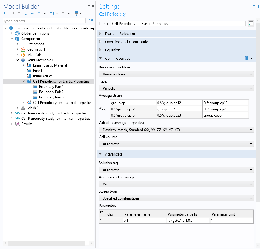 The Model Builder with the Cell Periodicity feature selected and the corresponding settings.
The Cell Periodicity feature.
The use of periodic boundary conditions for finding homogenized elastic properties is well known. However, the periodic conditions are not limited to the computation of homogenized elastic properties, but can be used to find homogenized thermal, hygroscopic, elastoplastic, viscoelastic, piezoelectric, or even electrical properties.
Homogenized Elastic Properties
The elastic constitutive law for a homogeneous or pseudohomogeneous material is written as

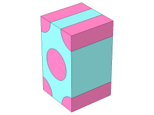
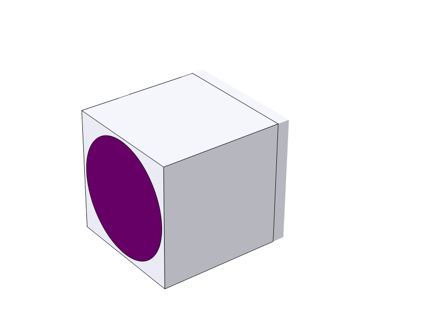
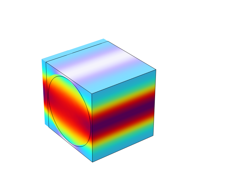
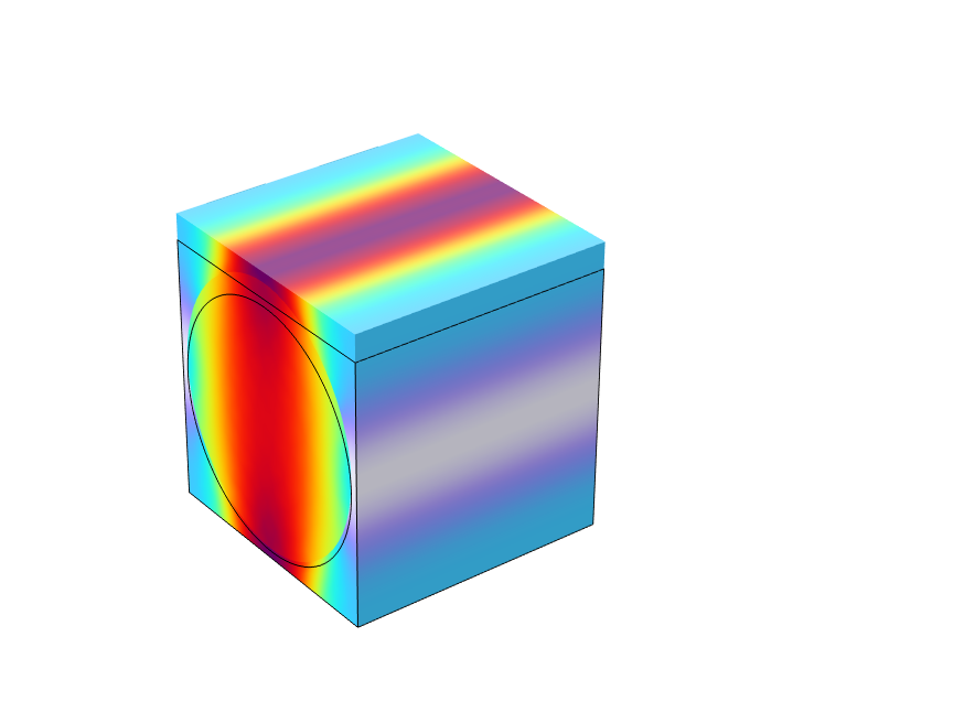
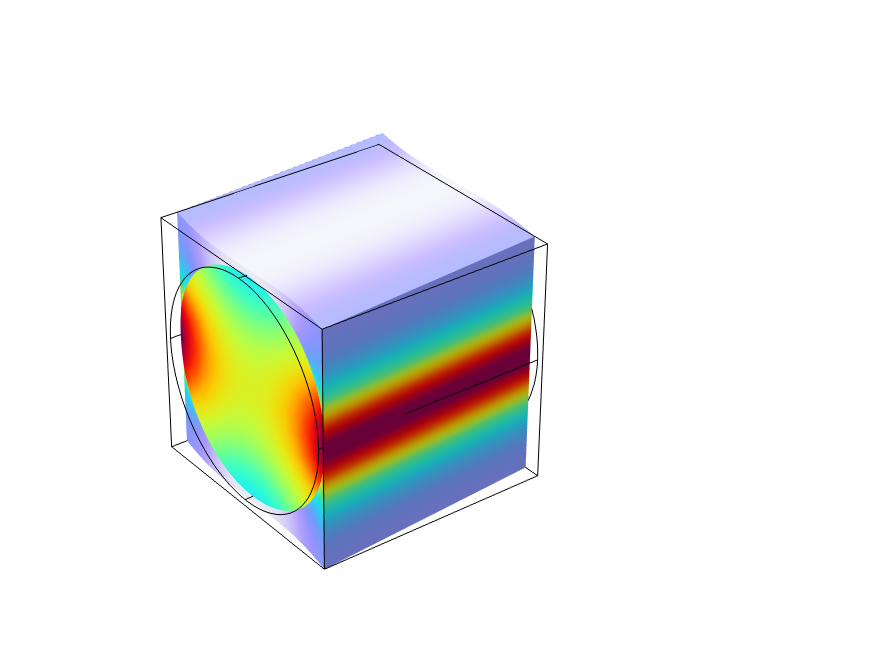
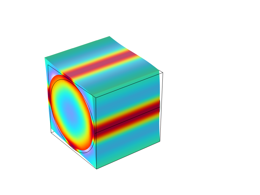
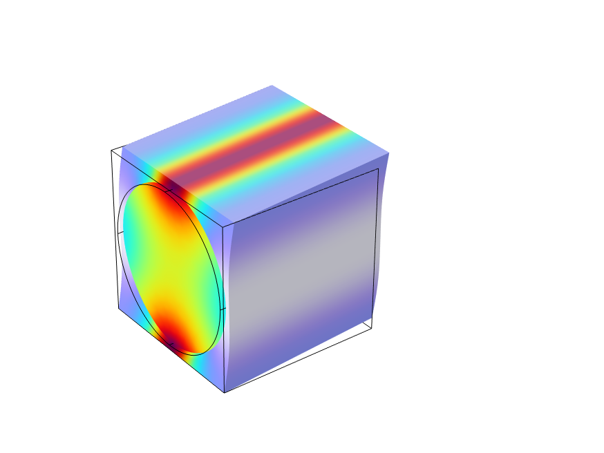
where  is the homogenized elasticity tensor. To find the components of the homogenized elasticity tensor using the periodic boundary conditions, six load cases are required. In each load case, one strain component is prescribed while the others are zero. The six fundamental load cases are shown below using an example with a unidirectional fiber composite.
 |
 |
 |
|---|---|---|
Load Case 1:  |
Load Case 2:  |
Load Case 3:  |
 |
 |
 |
Load Case 4:  |
Load Case 5:  |
Load Case 6:  |
Equivalent stress distribution for each of the unit strain cases.
The numerically computed homogenized material properties of a unidirectional fiber composite can be compared against the results from the analytical models available in the Effective Material node. See the Micromechanical Model of a Fiber Composite tutorial model for more details (results of the analysis are shown below).
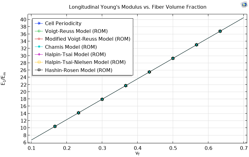 A graph showing the longitudinal Young's modulus versus the fiber volume fraction for different methods.
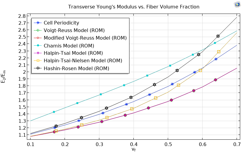 A graph showing the transverse Young's modulus versus the fiber volume fraction for different methods.
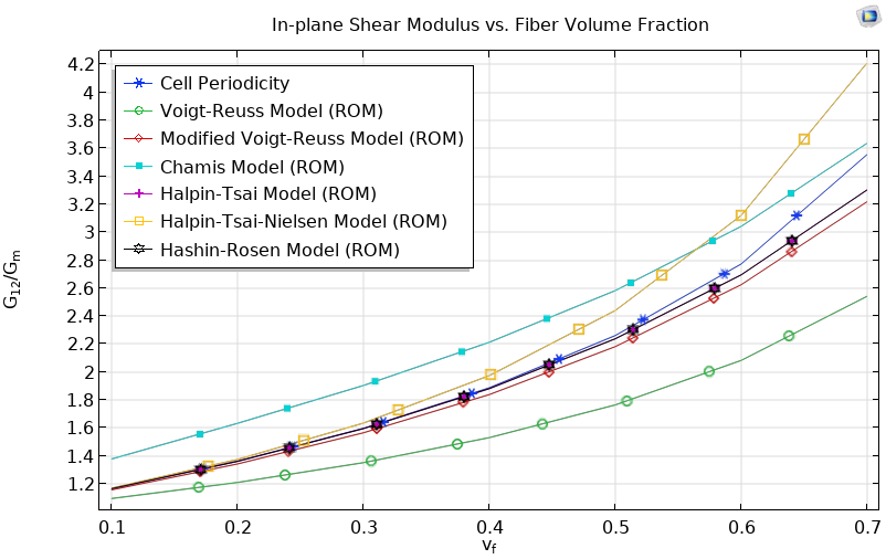 A graph showing the in-plane shear modulus versus the fiber volume fraction for different methods.
Effective Young's and shear moduli computed using analytical and numerical methods as functions of fiber fraction.
The longitudinal Young’s modulus matches quite closely between numerical and analytical models. The transverse Young’s modulus differs more and more as the fiber volume fraction increases. When comparing the analytical models, the results of the Halpin–Tsai–Nielsen model has the best match with the numerical results. For the in-plane homogeneous shear modulus, the Modified Voigt–Reuss model, Halpin–Tsai model, and Hashin–Rosen model give good results, while for small to medium volume fractions, the Halpin–Tsai-Nielsen model also matches the numerical results well. Thus, in all cases the Halpin–Tsai–Nielsen model gives good results for small to medium fiber volume fraction. It is important to acknowledge that analytical models are based on certain assumptions, which may not necessarily reflect real-world scenarios. Nonetheless, they can serve as valuable references for comparing numerical results.
The homogenization method shown here for a unidirectional fiber composite can be straightforwardly applied to other unit cells with complex geometry. Consider the example of a triply-periodic-minimal-surface-based (gyroid TPMS) composite, where the reinforcement in the matrix has a complex geometry. Such structures can, for example, be auxetic (i.e., have a negative Poisson's ratio), even though all constituents have a positive value of Poisson's ratio. The Micromechanical Model of a Triply-Periodic-Minimal-Surface-based Composite example shows the effect of negative Poisson's ratio and the volume fraction of TPMS material on the homogenized elastic and thermal properties of a composite.
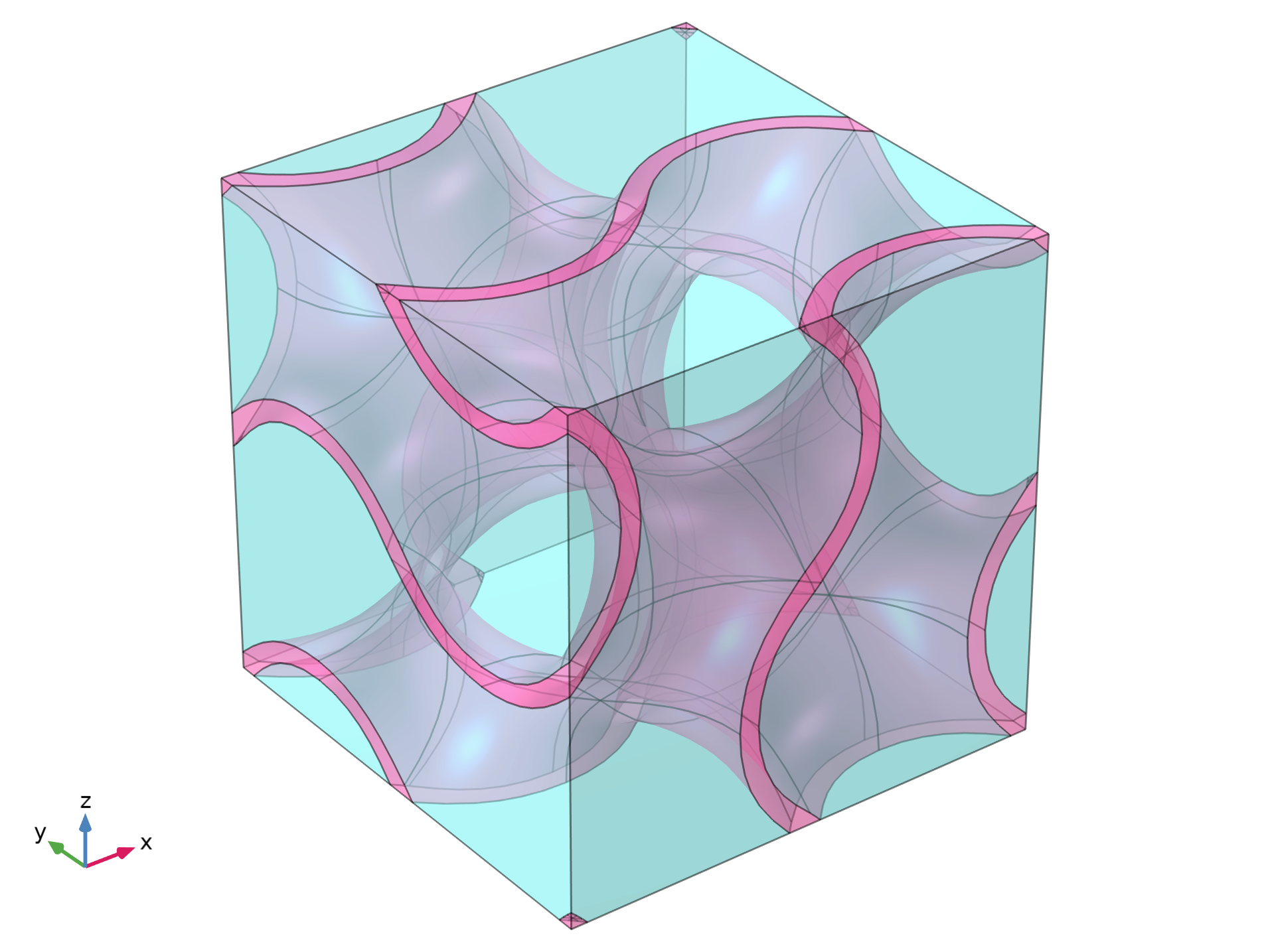
Unit cell of TPMS-based gyroid.
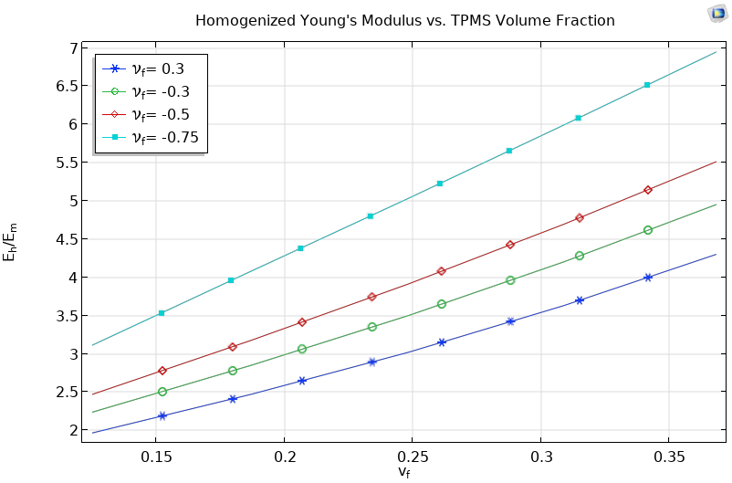 A graph showing the homogenized Young's modulus versus the TPMS volume fraction.f
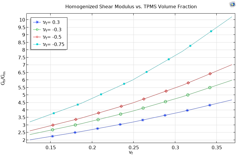 A graph showing the homogenized shear modulus versus the TPMS volume fraction.
Numerically computed effective Young's and shear moduli.
Homogenized Thermal or Hygroscopic Expansion Properties
The periodic boundary conditions of the Cell Periodicity feature can also be used to find the effective coefficient of thermal expansion or coefficient of hygroscopic swelling. The Micromechanical Model of a Fiber Composite tutorial model shows the computation of the effective coefficient of thermal expansion by analytical and numerical methods. For a range of volume fractions, the computed value in the longitudinal direction matches with the effective properties predicted by the analytical models. In the transverse direction, the numerical and analytical results differ significantly.
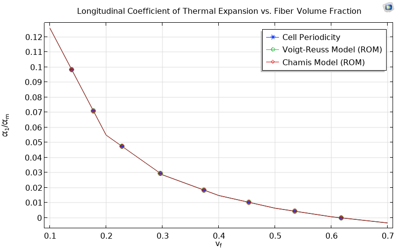 A graph showing the longitudinal coefficient of thermal expansion versus the fiber volume fraction.
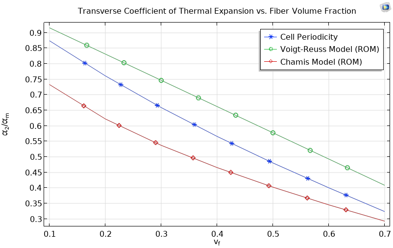 The transverse coefficient of thermal expansion versus the fiber volume fraction.
Effective coefficient of thermal expansion by analytical and numerical methods.
The Micromechanical Model of a Composite with Temperature-Dependent Properties tutorial model shows the computation of effective thermal properties as a function of temperature. In many real-life applications, the properties of constituent materials depend on the operating temperature, which in turn affects the effective properties of composite materials. Again, the numerical and analytical approaches have a good match in the longitudinal direction but differ in the predictions for the transverse direction.
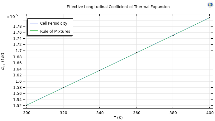 A graph showing the effective longitudinal coefficient of thermal expansion.
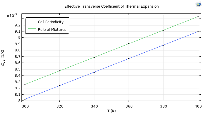 A graph showing the effective transverse coefficient of thermal expansion.
Effective coefficient of thermal expansion by analytical and numerical methods as functions of temperature.
Homogenized Viscoelastic Properties
Even though fiber composites are most commonly used, other types, such as particulate composites, are also used in different areas of technology. One important application of particulate composites is shock-absorbing and shock-resisting structures. For most particulate composites, both the particulates and matrix materials are isotropic. The effective anisotropic material properties are the effect of the particle distribution and positioning within the matrix.
In this example, we will look at the Micromechanical Model of a Particulate Composite model, a case where elastic particles are embedded in a viscoelastic matrix. The Cell Periodicity feature together with methods from the Optimization Module are used to compute the effective viscoelastic properties.
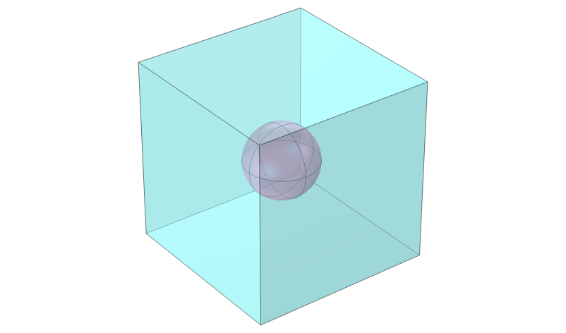
Unit cell of a particulate composite.
In an initial study, the long-term effective elastic properties are determined. Then, the composite microstructure (RUC) is subjected to transient shear and normal loading, which yields the viscoelastic response of the composite. This viscoelastic response is used to determine the effective viscoelastic properties of the homogenized material using curve fitting optimization. Finally, the results are validated by comparing the transient response of the heterogeneous material and the homogenized material.
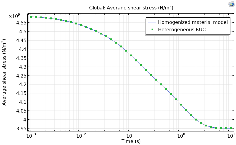 A graph showing the global average shear stress.
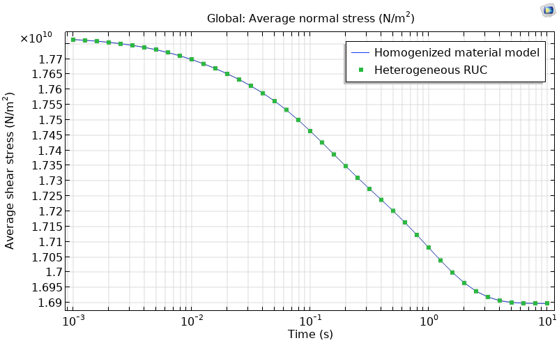 A graph showing the average normal stress.
Transient response of a heterogeneous and homogeneous microstructure to shear and normal loading, respectively.
Homogenized Piezoelectric Properties
Advancement of technology demands development of smart composites made of piezoelectric materials. The use of piezoelectric composites can be found in, for example, sensors, actuators, and transducers. In order to determine the response of such structures, a complete set of homogenized piezoelectric constitutive properties is needed. The periodic boundary conditions can be extended for the computation of the effective piezoelectric properties. The piezoelectric material's constitutive law needs elasticity or compliance matrix, coupling matrix, and relative permittivity. To determine these effective properties, three extra load cases containing the electric potential need to be added to the original six load cases for strain. The displacement periodic boundary conditions are part of the Cell Periodicity feature in the Solid Mechanics interface, while the electric potential periodic boundary conditions can be added using the Pointwise Constraint features in the Electrostatics interface. Because the problem involves a coupling between two different fields, the built-in multiphysics interface Piezoelectricity, Solid is used. The details can be found in the Micromechanical Model of a Piezoelectric Fiber Composite tutorial model.
Unit cell of a fiber composite. Fibers are made of PZT-7A material, while the matrix is made of barium titanate.
Homogenized Thermal Properties
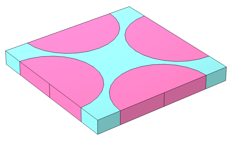
The Periodic Condition feature in the Heat Transfer in Solids interface can be used to computed homogenized heat capacity and thermal conductivity properties. The Homogenized Material Properties of Periodic Microstructures app shows how to compute the effective thermal properties with different unit cells.
Applications for Homogenization
The simulation applications (apps) developed in COMSOL Multiphysics® using the Application Builder are powerful yet simple simulation tools that truly democratize the simulation process. Such apps can be important for the case of homogenization where engineers are interested in the homogenized material properties directly rather than the underlying complex model setup. The user interface (UI) of such an app is much simpler than that of the underlying model. It is easy to compute homogenized material properties for different combinations of materials and microstructures.
The homogenized material properties of composite materials can be altered by choosing different microstructures, different constituent materials, and different volume fractions of the reinforcement phase. This gives many possible combinations to test. In such a scenario, homogenization apps based on the periodic boundary conditions in different physics interfaces provide flexibility along with accuracy. The Homogenized Material Properties of Periodic Microstructures app, developed in COMSOL Multiphysics® using the Application Builder, can be used to find the effective properties using different unit cells. The app has 10 built-in unit cells, with options to compute the effective density, elasticity tensor, coefficient of thermal expansion, heat capacity, and thermal conductivity. The effective material properties can be seen in the UI, but they can also be exported as a material file that can later be imported into another model.
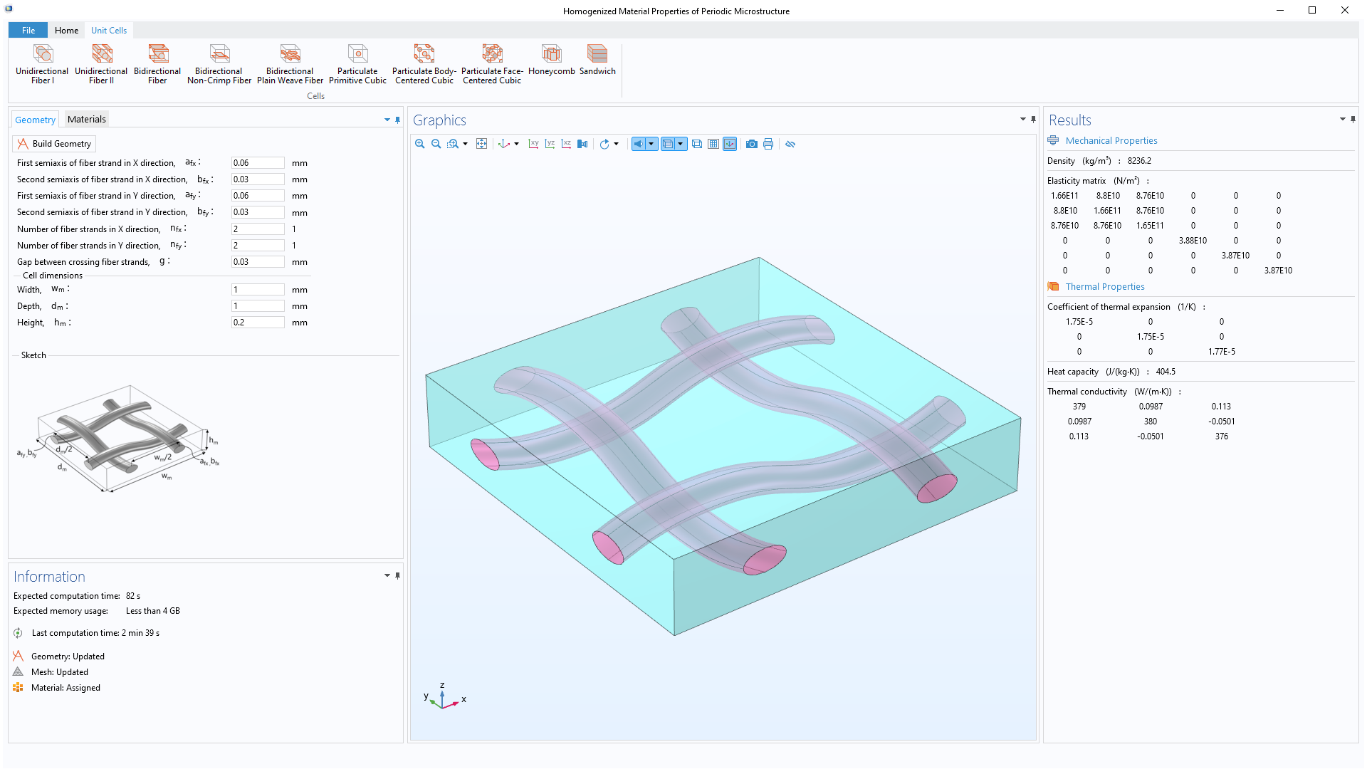 The UI of the Homogenized Material Properties of Periodic Microstructure app showing the model in the Graphics window as well as the Results window.
The UI of homogenization app showing computed homogenized material properties for bidirectional plain weave fiber composite.
So far, we have talked about homogenization in solids using periodic boundary conditions applied on an RUC. But what happens if the material microstructure is not periodic, e.g., having randomly distributed particles in the matrix? For such materials, the material subvolume must be analyzed as an RVE, and homogeneous boundary conditions must be applied to estimate the homogenized material properties. The Cell Periodicity feature in the Solid Mechanics interface provides the possibility to also apply homogeneous boundary conditions, which are discussed in the next section.
Homogeneous Boundary Condition
The homogeneous boundary condition is written as
 .
.
Similarly, the homogeneous traction condition is written as
 ,
,
where  is the traction,
  is the macroscopic stress, and
  is the material normal.
The homogeneous boundary conditions should be used on an RVE subvolume, while the periodic boundary conditions are appropriate for an RUC subvolume. What will then determine the choice between RVE and RUC? When the microstructure of the material is truly periodic, periodic boundary conditions will give the most accurate results. If homogeneous boundary conditions are applied to a periodic structure, they will produce apparent material properties that asymptotically approach the effective material properties obtained using periodic boundary conditions when the number of unit cells is increased. The convergence is either from below or above, depending on whether displacement or traction boundary conditions are used (Ref. 2). If one constituent is randomly distributed in another constituent, then the microstructure is not periodic. In this case, homogeneous boundary conditions should be used. When using homogeneous boundary conditions, one must keep in mind that the size of the RVE affects the effective properties. The size of the RVE can be considered sufficient if it gives the same results with the displacement and traction boundary conditions.
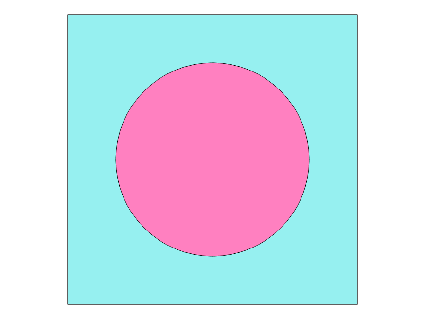
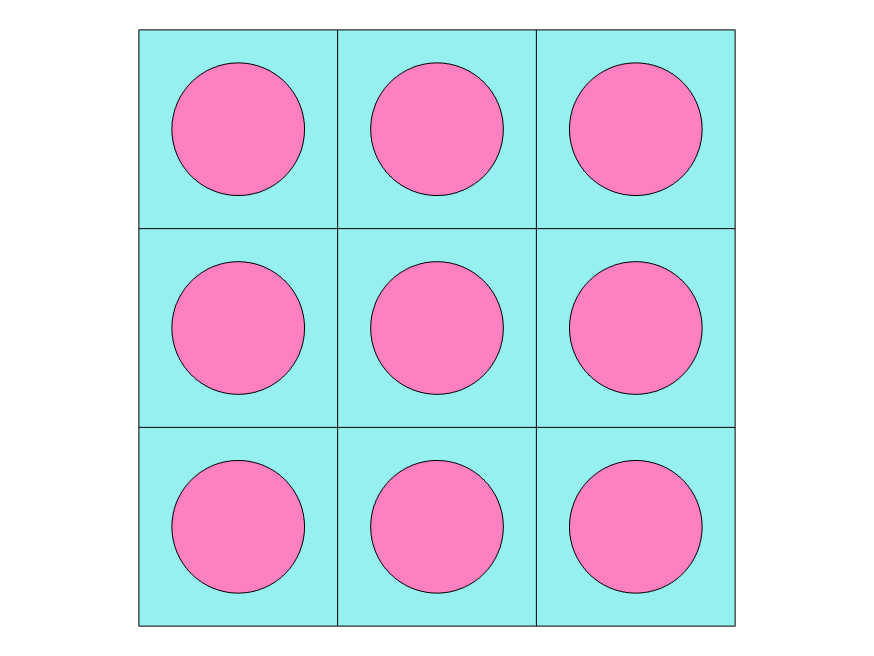
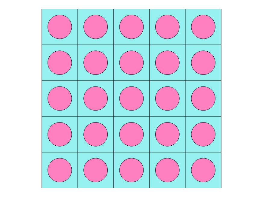
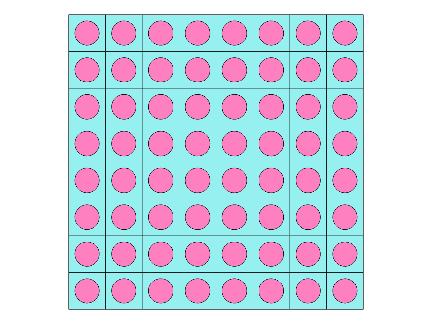
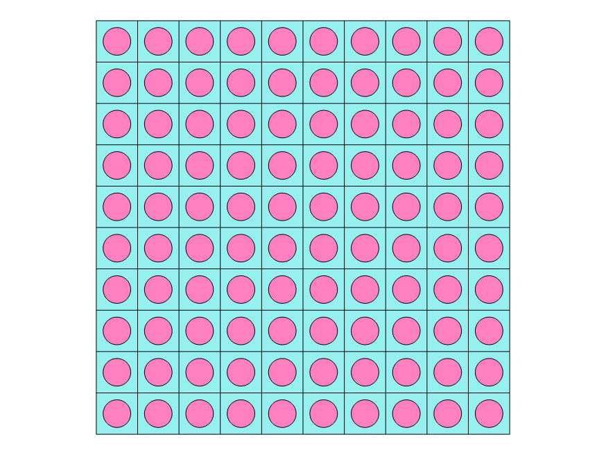
To show the impact of boundary conditions on the effective properties, an example from Reference 2 is used. The aim of the example is to find the effective properties of a unidirectional fiber composite with homogeneous and periodic boundary conditions when different sizes of the subvolume are used. Here, we are not calling the subvolume either RVE or RUC since both are valid terms depending on the boundary conditions used. The different sizes of the subvolumes are shown in the figures below.
The Micromechanical Analysis with Homogeneous and Periodic Boundary Conditions example can be found in the Application Gallery.
 |
 |
 |
 |
 |
|---|---|---|---|---|
| 1 unit cell | 3 x 3 unit cells | 5 x 5 unit cells | 8 x 8 unit cells | 10 x 10 unit cells |
Material subvolume with a different number of unit cells.
Changing the number of unit cells in the material subvolume does not affect the effective properties computed with periodic boundary conditions. It does, however, have an impact on the effective properties computed using homogeneous boundary conditions. The results are presented below.
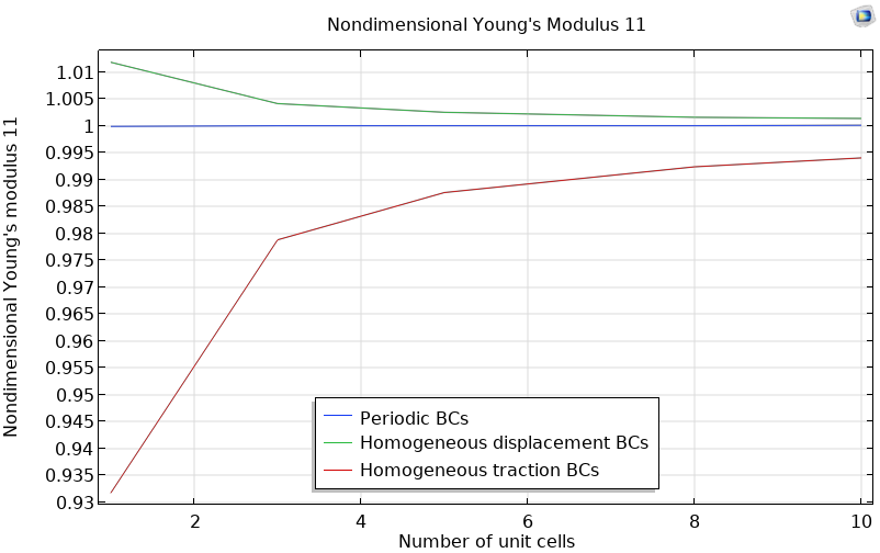 A graph plotting the nondimensional Young's modulus and a number of unit cells.
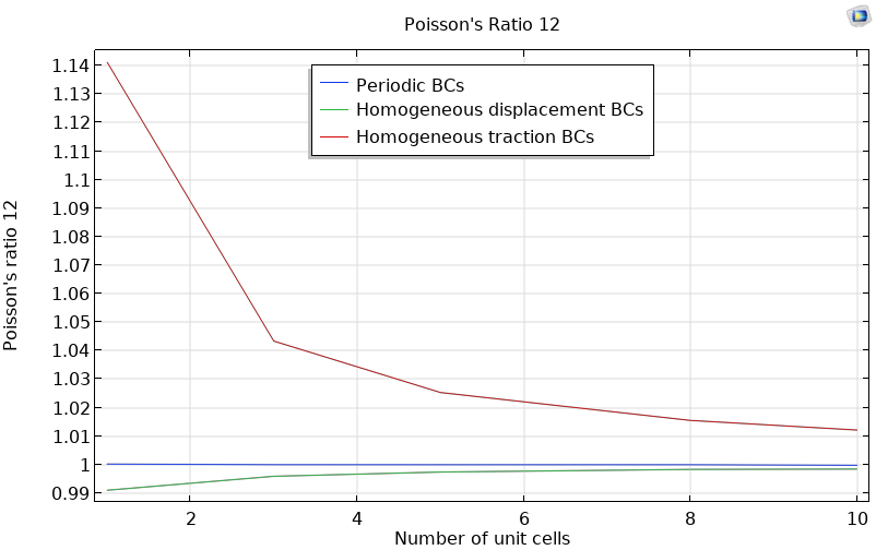 A graph plotting the Poisson's ratio and a number of unit cells.
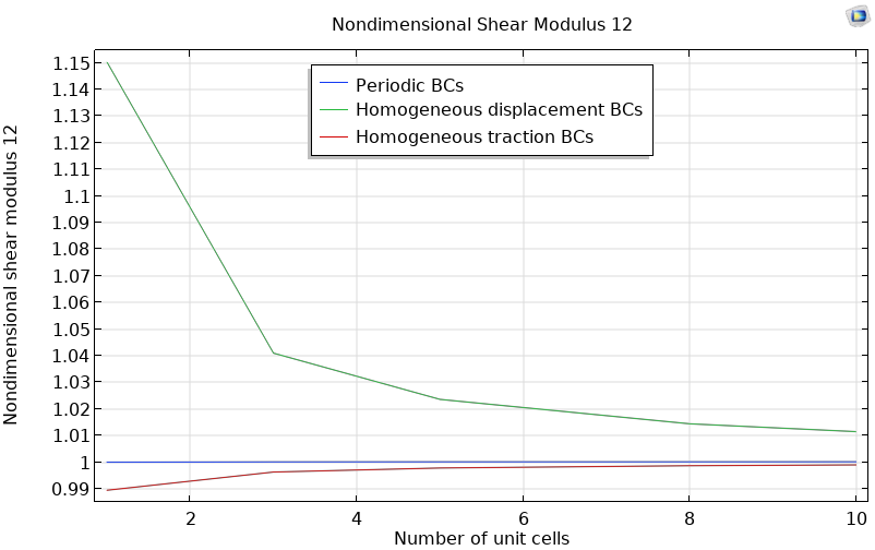 A graph plotting the nondimensional shear modulus and number of unit cells.
The effective material properties using different number of unit cells in a material subvolume with homogeneous and periodic boundary conditions.
As expected, the apparent Young's and shear moduli of heterogeneous subvolumes under homogeneous displacement and traction boundary conditions approach the effective moduli under periodic boundary conditions from above and below, respectively, when the number of cells is increased. For Poisson's ratio, the trend is the opposite.
To summarize, the periodic boundary condition can be used when the microstructure of the material is truly periodic, while the homogeneous boundary conditions are used when the microstructure is not periodic but random distribution of constituents.
Homogenization in Shells
In finite element analysis, thin structures with in-plane dimensions that are larger than the thickness can be treated using shell elements, corresponding to the Shell interface in COMSOL Multiphysics®.
With a linear elastic material, the relation between section forces and strain for a shell with a symmetric profile about midplane is written as


 ,
,
where
 ,
,  ,
,  are the in-plane force, in-plane moment, and out-of-plane shear force resultants.
 ,
,  ,
,  are the membrane, bending, and shear part of the strain tensor.
 ,
,  ,
,  are the extensional, shear, and bending stiffness matrices.
  is the shear correction factor.
The stiffness matrices are derived from the integration of the elasticity tensor over the thickness. This is also a kind of homogenization at the mesoscale (intermediary scale between the micro and macro scale). Using the Shell interface, a layered composite plate can be treated as an equivalent single layer plate.
Another kind of homogenization done for thin structures is when a corrugated or perforated sheet is treated as an equivalent orthotropic sheet. Here, the material is monolithic, while there is a periodicity in the geometry. Periodic boundary conditions are applied to the corrugated sheet to get the equivalent stiffness matrices. These equivalent stiffness matrices can then be used directly in a Section Stiffness material model in the Shell interface using a simplified flat geometry. Note that in the Shell interface there is no feature similar to Cell Periodicity, so the periodic boundary conditions need to be applied using Prescribed Displacement nodes. The constitutive relation for an equivalent orthotropic plate is written as


 ,
,
where over-bar quantities are equivalent (or macroscopic or average) quantities.
To find these effective stiffness matrices, eight load cases are needed, where in each load case all strain components are zero except the one strain component that is unity. The authors in References 3–5 have proposed analytical formulas for different stiffness components for different corrugated sheets. The load cases for obtaining effective transverse shear stiffness are not possible to model using only shell theory. It would be necessary to use the Solid Mechanics interface. In the Homogenized Model of a Corrugated Sheet example, the equivalent A and D stiffness matrices for trapezoidal and round corrugated sheets are computed numerically and the results are compared with the analytical formulas. Unit cells for different corrugations are available as geometry parts in the RVEs and Unit Cells folder under the COMSOL Multiphysics folder.
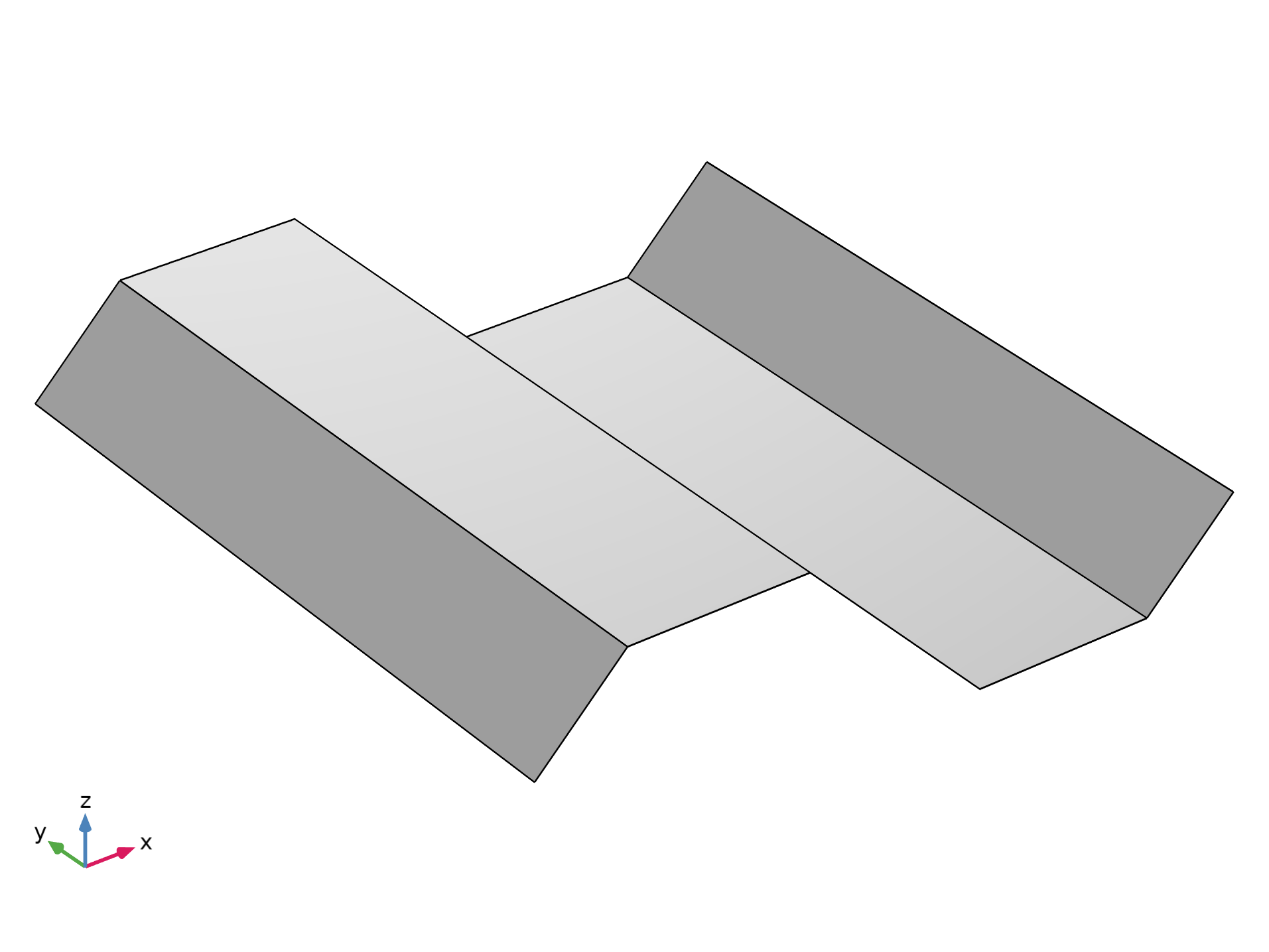
Unit cell of a trapezoidal corrugation.
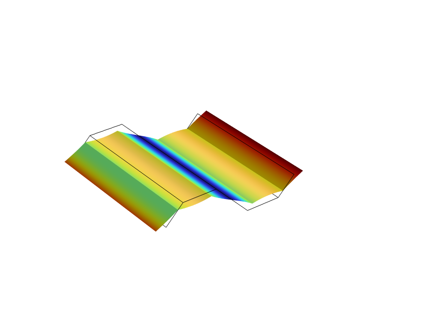
For the trapezoidal corrugation example, the three load cases corresponding to in-plane membrane strains and three load cases corresponding to bending strains are shown below.
 |
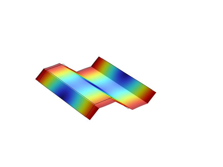 |
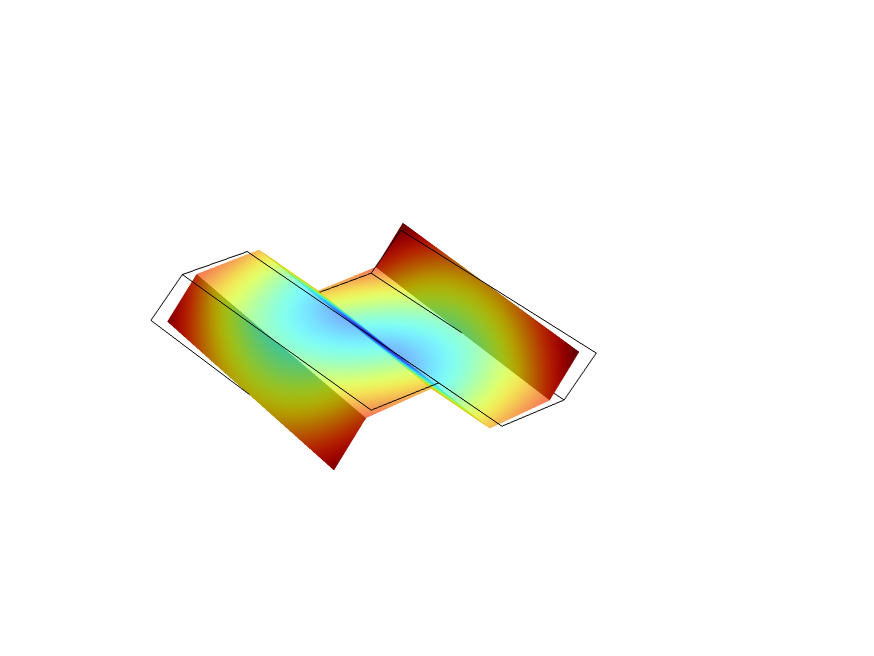 |
|---|---|---|
Load Case 1:  |
Load Case 2:  |
Load Case 3:  |
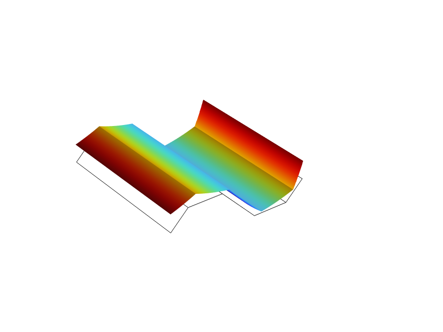 |
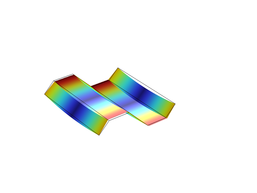 |
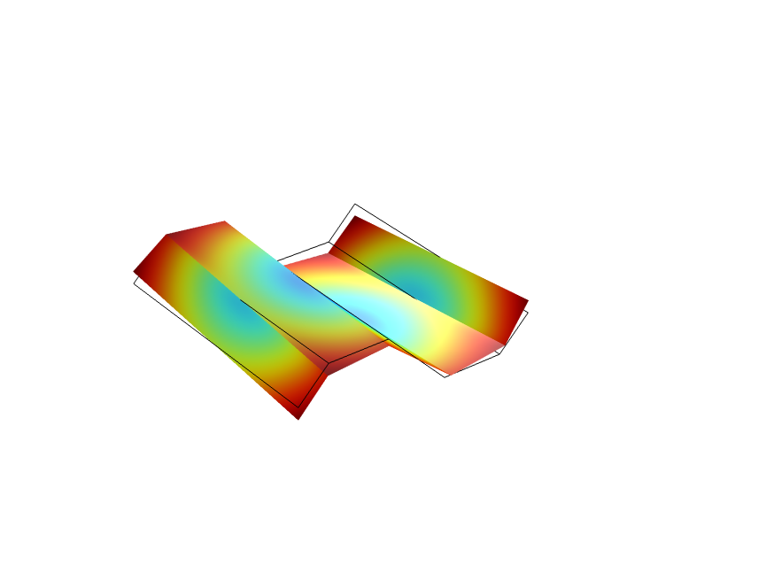 |
Load Case 4:  |
Load Case 5:  |
Load Case 6:  |
The numerical effective stiffness components are computed based on the reaction forces and energy equivalence. The numerical values of stiffness components computed based on the energy equivalence approach returns same values as the approach based on the reaction forces. The analytical and numerical values of the stiffness components for a trapezoidal corrugation are given in the table below.
| Stiffness Component | Ref. 3 | Numerical: Based on Reactions |
|---|---|---|
 |
3.92 | 3.92 |
 |
1.17 | 1.17 |
 |
161 | 161 |
 |
42.4 | 42.4 |
 |
407.6 | 407.9 |
 |
122.3 | 120.8 |
 |
17809 | 16237 |
 |
208.0 | 180.6 |
It should be noted that the analytical values for some of the stiffness coefficients are based on assumptions that are not exactly fulfilled in reality, so the numerical values should be considered as more correct.
The equivalent stiffness matrices for the round corrugation sheet are also computed and compared with the analytical values from Reference 3 in the same example. The boundary conditions presented in the example can be straightforwardly extended to the multilayered corrugated sheets or flat perforated sheets.
Homogenization in Beams
A structure that has one dimension much larger than the other two dimensions can be analyzed using beam elements. In COMSOL Multiphysics®, the Beam interface can be used for this purpose. In this section, we limit our discussion to the Euler–Bernoulli beams. With the linear elastic constitutive relation, the section forces–strain relation for a beam is written as

where index 1 refers to the axial direction and indices 2 and 3 are the local lateral directions of the beam.  is the extension of the reference line,
  is the elastic twist, and
  and
and  are the elastic bending curvatures.
  is the axial force in the section,
  is the twisting moment in the cross section, and
  and
and  are the bending moments.
The Beam interface does not model the cross section of the structure explicitly. This means that if the cross section is made of multiple materials (for example, a composite beam), then it is not possible to model it unless homogenization methods are used to obtain an equivalent stiffness. Such an equivalent stiffness can later be used in the Section Stiffness material model in the Beam interface. The constitutive relation for the homogenized beam is written as

where over-bar quantities are equivalent (macroscopic, or average) quantities.
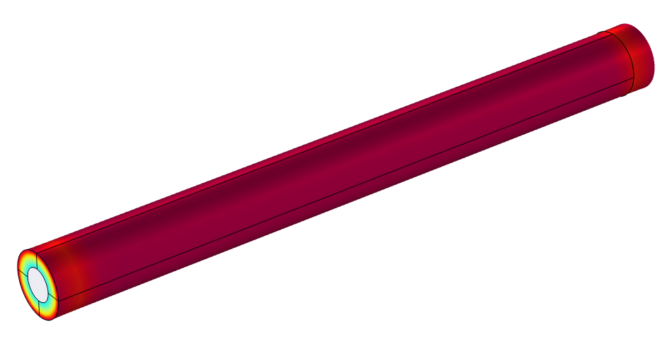
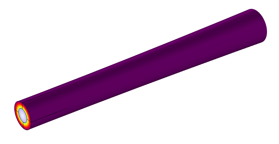
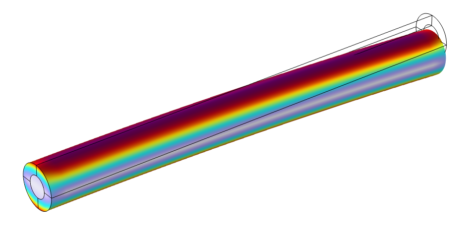
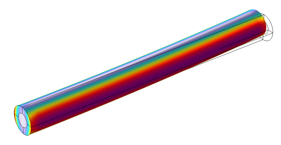
The true multimaterial beam cannot be represented in the Beam interface, so the Solid Mechanics interface needs to be used for a homogenization of beam properties. The prescribed displacement functionality of the Rigid Connector feature is used to keep the beam cross-section plane during the deformation. This is a basic assumption of the Euler–Bernoulli theory. To get all the components of the equivalent stiffness matrix, four load cases are required. The first is axial extension and the remaining three are twisting and bending load cases.
See the Homogenization of a Composite Beam model for the implementation details. In this example, a circular beam made of two different materials is considered. The effective stiffness obtained after homogenization can used with the Section Stiffness material model in the Beam interface.
 |
 |
 |
 |
|---|---|---|---|
Load Case 1:  |
Load Case 2:  |
Load Case 3:  |
Load Case 4:  |
The numerical values of the stiffness components for the composite beam are written in the table below.
| Stiffness Component | Numerical |
|---|---|
 |
337.96 |
 |
45.258 |
 |
60.112 |
 |
60.112 |
Note that for this simple beam, there is not coupling between the different types of action. In general, this is not the case.
Once the effective stiffness matrix is obtained, the next step is to verify it by comparing the homogenized beam model modeled in the Beam interface with a corresponding heterogeneous beam modeled using the Solid Mechanics interface. Three point forces and three point moments are used to evaluate the response using six separate load cases. The results obtained with the Beam interface are compared with results from the Solid Mechanics interface. The tip displacement of the homogenized beam (modeled with the Beam interface) and heterogeneous beam (modeled with the Solid Mechanics interface) for all load cases are shown below.
| Tip Displacement/Rotation | Load Case 1  |
Load Case 2  |
Load Case 3  |
Load Case 4  |
Load Case 5  |
Load Case 6  |
|---|---|---|---|---|---|---|
 |
2.958 | 0 | 0 | 0 | 0 | 0 |
 |
0 | 55.45 | 0 | 0 | 0 | 8.317 |
 |
0 | 0 | 55.45 | 0 | -8.317 | 0 |
 |
0 | 0 | 0 | 2.209 10-5 10-5 |
0 | 0 |
 |
0 | 0 | -8.31710-5 |
0 | 1.663610-5 |
0 |
 |
0 | 8.31710-5 |
0 | 0 | 0 | 1.663610-5 |
Tip displacement and rotations in the homogenized Beam interface.
| Tip Displacement/Rotation | Load Case 1 |
Load Case 2 |
Load Case 3 |
Load Case 4 |
Load Case 5 |
Load Case 6 |
|---|---|---|---|---|---|---|
|
3.032 | 0 | 0 | 0 | 0 | 0 |
|
0 | 56.36 | 0 | 0 | 0 | 8.458 |
|
0 | 0 | 56.36 | 0 | -8.458 | 0 |
|
0 | 0 | 0 | 2.20910-5 |
0 | 0 |
|
0 | 0 | -8.45810-5 |
0 | 1.695010-5 |
0 |
|
0 | 8.45810-5 |
0 | 0 | 0 | 1.695010-5 |
Average tip displacement and rotations in the Solid Mechanics interface.
Based on both tables it is clear that there is a good match between the Beam and Solid Mechanics results, which indicates the correctness of the homogenization method employed for the composite beam.
A few important things must be noted in the case of beam homogenization:
- If the location of the shear center differs from the geometric center, then it must be taken into account in the Section Stiffness material model. It also needs to be considered when applying loads.
- If the composite beam has a different shear center location than the geometric center, then there is coupling between torsion and the bending.
The example shown here has a beam with a circular cross section that is made of two different materials, with an axially symmetric distribution. The shear center is then identical to the geometric center, so these complications are avoided.
Concluding Remarks
Homogenization is a powerful technique that makes it possible to treat a heterogeneous material or structure as homogeneous at a global scale, making analysis feasible without sacrificing accuracy. With the advancement of technology, composite materials and structures have become increasingly popular. A structured application of homogenization methods will simplify the complex material systems and make the simulation faster at a global scale, thus fostering innovation.
References
- J. Aboudi, S.M. Arnold, B.A. Bednarcyk, Micromechanics of Composite Materials: A Generalized Multiscale Analysis Approach, Elsevier, First Edition, 2013.
- A. Drago and M.J. Pindera, "Micro-macromechanical analysis of heterogeneous materials: Macroscopically homogeneous vs. periodic microstructures," Composites Science and Technology, vol. 67, no. 6, pp. 1243–1263, 2007.
- K.J. Park, K. Jung, and Y.W. Kim, "Evaluation of homogenized effective properties for corrugated composite panels," Composite Structures, vol. 140, pp. 644–654, 2016.
Submit feedback about this page or contact support here.