Fitting the Debye Dispersion Model to Experimental Data
This article addresses how to use the Partial Fraction Fit function in COMSOL Multiphysics® to fit a Debye dispersion model to experimental data. This functionality is available as of versions 6.2 of the software.
Background
When modeling the electrical response of materials in the frequency and time domain, it can be important to consider the variation in the relative permittivity as a function of frequency. This material data is experimentally determined and usually presented as the real and the negative imaginary component of the relative permittivity:

The negative imaginary component corresponds to loss. It is common to present the magnitude of the imaginary term, since the data is often plotted in the log–log scale. The plot below shows sample data, which is also available from the supporting data file.
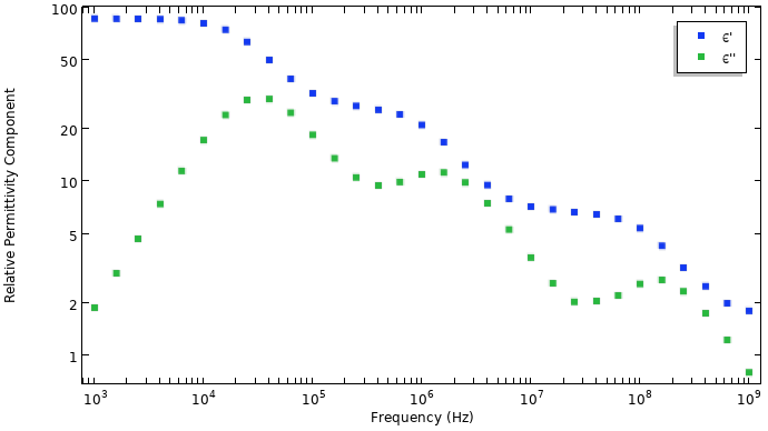 Sample experimental data consisting of the real component of the permittivity and the magnitude of the negative imaginary component.
This type of data has two issues:
It cannot be used within a time-domain model. If there is any kind of experimental error in the data, then it can produce noncausal results. So, rather than using this experimental data directly, a Debye material model is fit to the data, and that material model is used instead. The Debye model can be used in a time-domain model, and it satisfies the Kramers–Kronig relations, so the results will be causal.
The Debye model defines the complex-valued permittivity with respect to angular frequency,  , as:
, as:
 ,
,
which takes as input any number,  , of poles where each pole,
  , has a relaxation time,
  , and relative permittivity contributions,
  , as well as the high-frequency limit,
  . Once these model parameters are known, they can be used within both frequency- and time-domain models.
This article describes how to work with the experimental data in a text file form, fit a Debye model to it, and extract the model parameters.
Workflow
The experimental data is fit using the Partial Fraction Fit function. This feature can be added to Global Definitions > Functions and within Component > Definitions > Functions. The screenshot below shows the interface as the experimental data is read from a text file.
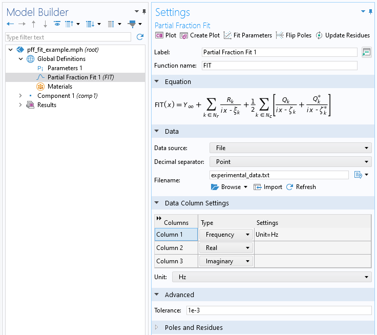 Screenshot of the Partial Fraction Fit function as the data is imported from a text file.
Once the data is imported, click the Fit Parameters button. This will fit to the data a complex-valued function of the form:
 ,
,
where  can be complex-valued,
  and
and  are the
  number of real-valued residues and poles, and
  and
and  are the
  number of complex-valued residues and poles. Note that the argument to the function,
  , has units of hertz, not angular frequency. The quality of the fit is governed by the Tolerance value in the Advanced setting. Tighter tolerances can significantly increase the time to compute the fit.
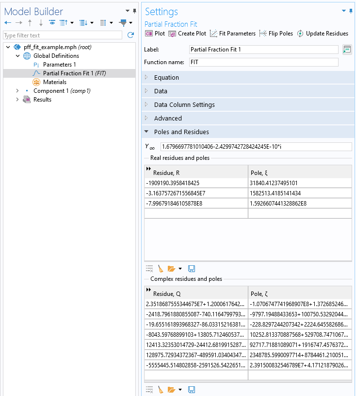 After Fit Parameters is clicked.
Note that since the imaginary component of the permittivity is entered in terms of its magnitude, rather than as negative numbers, the real poles will be positive rather than negative. It is possible to visually inspect the quality of the fit by creating a plot.
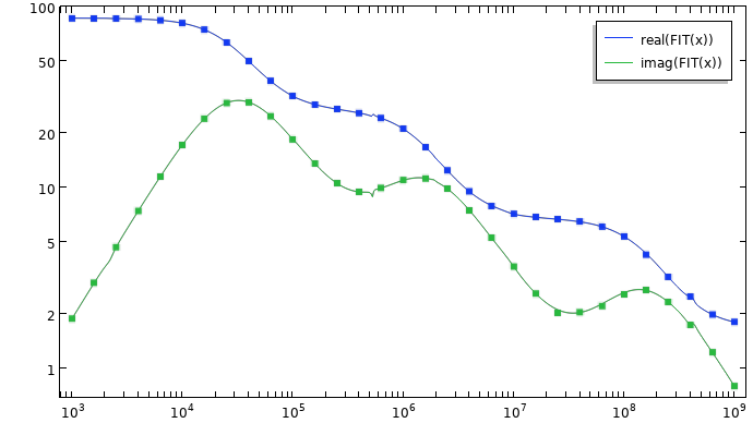 Plot of the experimental data and the partial fraction fit, including complex residues.
To match the Debye model, we are interested in those fits without complex-valued residues and poles. It is possible to ignore all of the complex-valued poles by using the Clear Table option. After this table is cleared, click the Update Residues button, which will leave the real-valued poles unchanged but update the real-valued residues.
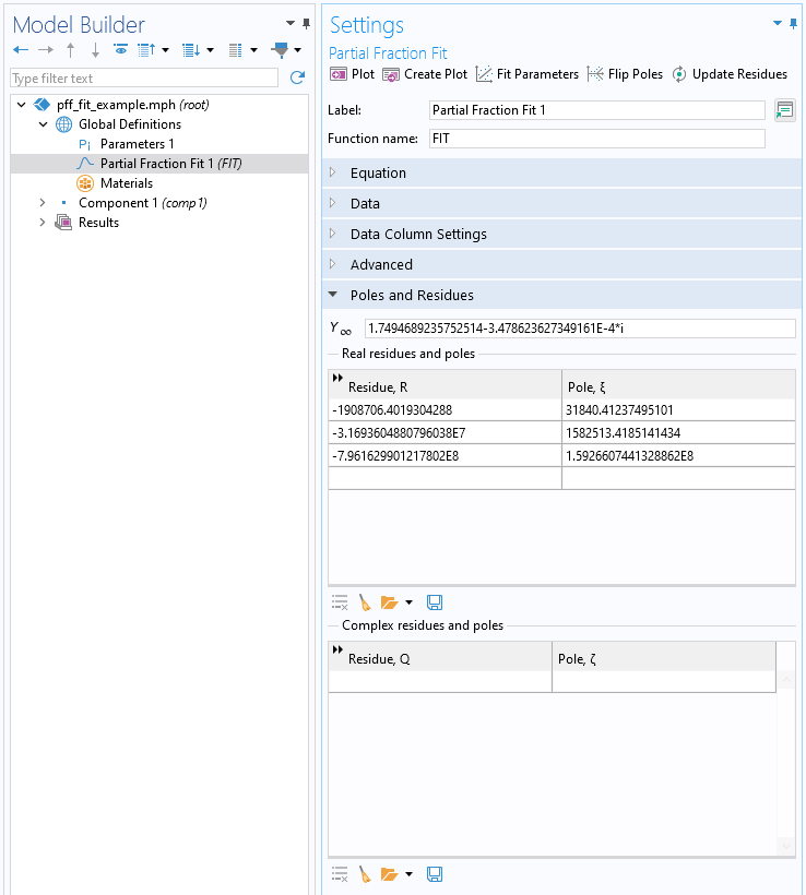 Screenshot after clearing the table of complex-valued residues and poles and updating the remaining real-valued residues.
 Plot of the fit to the experimental data, using only the real-valued poles and updated residues.
The real poles of the fit correspond to the Debye model relaxation times,
 .
.
The residues and poles correspond to the Debye model relative permittivity contributions,
 .
.
Lastly, the term can be complex-valued, but if the imaginary component is relatively small, then the term of the Debye model corresponds to:
 .
.
These values can then be used within any of the Debye dispersion material model features in the software.
Submit feedback about this page or contact support here.