
In the second part of our Geothermal Energy series, we focus on the coupled heat transport and subsurface flow processes that determine the thermal development of the subsurface due to geothermal heat production. The described processes are demonstrated in an example model of a hydrothermal doublet system.
Deep Geothermal Energy: The Big Uncertain Potential
One of the greatest challenges in geothermal energy production is minimizing the prospecting risk. How can you be sure that the desired production site is appropriate for, let’s say, 30 years of heat extraction? Usually, only very little information is available about the local subsurface properties and it is typically afflicted with large uncertainties.
Over the last decades, numerical models became an important tool to estimate risks by performing parametric studies within reasonable ranges of uncertainty. Today, I will give a brief introduction to the mathematical description of the coupled subsurface flow and heat transport problem that needs to be solved in many geothermal applications. I will also show you how to use COMSOL software as an appropriate tool for studying and forecasting the performance of (hydro-) geothermal systems.
Governing Equations in Hydrothermal Systems
The heat transport in the subsurface is described by the heat transport equation:
(1)
Heat is balanced by conduction and convection processes and can be generated or lost through defining this in the source term, Q. A special feature of the Heat Transfer in Porous Media interface is the implemented Geothermal Heating feature, represented as a domain condition: Q_{geo}.
There is also another feature that makes the life of a geothermal energy modeler a little easier. It’s possible to implement an averaged representation of the thermal parameters, composed from the rock matrix and the groundwater using the matrix volume fraction, \theta, as a weighting factor. You may choose between volume and power law averaging for several immobile solids and fluids.
In the case of volume averaging, the volumetric heat capacity in the heat transport equation becomes:
(2)
and the thermal conductivity becomes:
(3)
Solving the heat transport properly requires incorporating the flow field. Generally, there can be various situations in the subsurface requiring different approaches to describe the flow mathematically. If the focus is on the micro scale and you want to resolve the flow in the pore space, you need to solve the creeping flow or Stokes flow equations. In partially saturated zones, you would solve Richards’ equation, as it is often done in studies concerning environmental pollution (see our past Simulating Pesticide Runoff, the Effects of Aldicarb blog post, for instance).
However, the fully-saturated and mainly pressure-driven flows in deep geothermal strata are sufficiently described by Darcy’s law:
(4)
where the velocity field, \mathbf{u}, depends on the permeability, \kappa, the fluid’s dynamic viscosity, \mu, and is driven by a pressure gradient, p. Darcy’s law is then combined with the continuity equation:
(5)
If your scenario concerns long geothermal time scales, the time dependence due to storage effects in the flow is negligible. Therefore, the first term on the left-hand side of the equation above vanishes because the density, \rho, and the porosity, \epsilon_p, can be assumed to be constant. Usually, the temperature dependencies of the hydraulic properties are negligible. Thus, the (stationary) flow equations are independent of the (time-dependent) heat transfer equations. In some cases, especially if the number of degrees of freedom is large, it can make sense to utilize the independence by splitting the problem into one stationary and one time-dependent study step.
Fracture Flow and Poroelasticity
Fracture flow may locally dominate the flow regime in geothermal systems, such as in karst aquifer systems. The Subsurface Flow Module offers the Fracture Flow interface for a 2D representation of the Darcy flow field in fractures and cracks.
Hydrothermal heat extraction systems usually consist of one or more injection and production wells. Those are in many cases realized as separate boreholes, but the modern approach is to create one (or more) multilateral wells. There are even tactics that consist of single boreholes with separate injection and production zones.
Note that artificial pressure changes due to water injection and extraction can influence the structure of the porous medium and produce hydraulic fracturing. To take these effects into account, you can perform poroelastic analyses, but we will not consider these here.
COMSOL Model of a Hydrothermal Application: A Geothermal Doublet
It is easy to set up a COMSOL Multiphysics model that features long time predictions for a hydro-geothermal application.
The model region contains three geologic layers with different thermal and hydraulic properties in a box with a volume V≈500 [m³]. The box represents a section of a geothermal production site that is ranged by a large fault zone. The layer elevations are interpolation functions from an external data set. The concerned aquifer is fully saturated and confined on top and bottom by aquitards (impermeable beds). The temperature distribution is generally a factor of uncertainty, but a good guess is to assume a geothermal gradient of 0.03 [°C/m], leading to an initial temperature distribution T0(z)=10 [°C] – z·0.03 [°C/m].
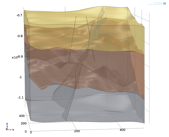
Hydrothermal doublet system in a layered subsurface domain, ranged by a fault zone. The edge is about 500 meters long. The left drilling is the injection well, the production well is on the right. The lateral distance between the wells is about 120 meters.
COMSOL Multiphysics creates a mesh that is perfectly fine for this approach, except for one detail — the mesh on the wells is refined to resolve the expected high gradients in that area.
")
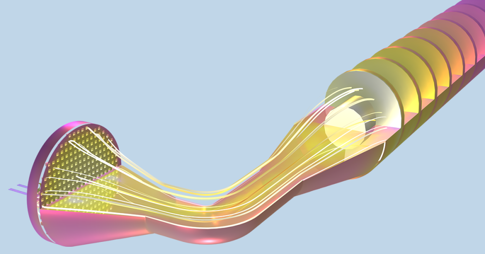
Now, let’s crank the heat up! Geothermal groundwater is pumped (produced) through the production well on the right at a rate of 50 [l/s]. The well is implemented as a cylinder that was cut out of the geometry to allow inlet and outlet boundary conditions for the flow. The extracted water is, after using it for heat or power generation, re-injected by the left well at the same rate, but with a lower temperature (in this case 5 [°C]).
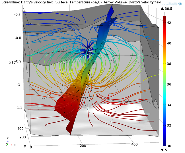
The resulting flow field and temperature distribution after 30 years of heat production are displayed below:
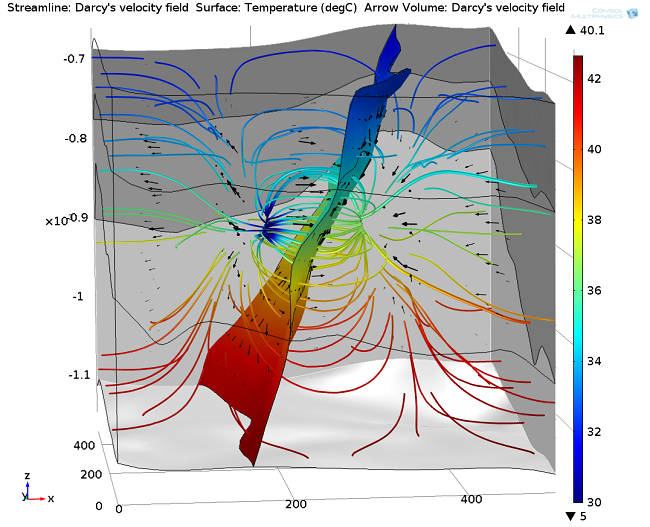
Result after 30 years of heat production: Hydraulic connection between the production and injection zones and temperature distribution along the flow paths. Note that only the injection and production zones of the boreholes are considered. The rest of the boreholes are not implemented, in order to reduce the meshing effort.
The model is a suitable tool for estimating the development of a geothermal site under varied conditions. For example, how is the production temperature affected by the lateral distance of the wells? Is it worthwhile to reach a large spread or is a moderate distance sufficient?
This can be studied by performing a parametric study by varying the well distance:
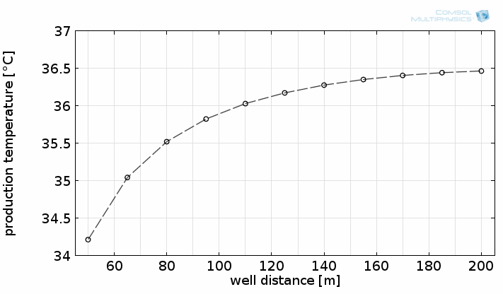
Flow paths and temperature distribution between the wells for different lateral distances. The graph shows the production temperature after reaching stationary conditions as a function of the lateral distance.
With this model, different borehole systems can easily be realized just by changing the positions of the injection/production cylinders. For example, here are the results of a single-borehole system:
Results of a single-borehole approach after 30 years of heat production. The vertical distance between the injection (up) and production (down) zones is 130 meters.
So far, we have only looked at aquifers without ambient groundwater movement. What happens if there is a hydraulic gradient that leads to groundwater flow?
The following figure shows the same situation as the figure above, except that now there is a hydraulic head gradient of \nablaH=0.01 [m/m], leading to a superposed flow field:
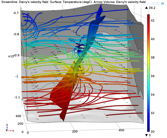
Single borehole after 30 years of heat production and overlapping groundwater flow due to a horizontal pressure gradient.
Other Posts in This Series
- Modeling Geothermal Processes with COMSOL Software
- Geothermal Energy: Using the Earth to Heat and Cool Buildings
Further Reading
- Download the Geothermal Doublet tutorial
- Explore the Subsurface Flow Module
- Related papers and posters presented at the COMSOL Conference:
- Hydrodynamic and Thermal Modeling in a Deep Geothermal Aquifer, Faulted Sedimentary Basin, France
- Simulation of Deep Geothermal Heat Production
- Full Coupling of Flow, Thermal and Mechanical Effects in COMSOL Multiphysics® for Simulation of Enhanced Geothermal Reservoirs
- Multiphysics Between Deep Geothermal Water Cycle, Surface Heat Exchanger Cycle and Geothermal Power Plant Cycle
- Modelling Reservoir Stimulation in Enhanced Geothermal Systems

Comments (31)
Bastiano Deschmann
May 30, 2015Where can I find the model file of this geothermal doublet?
Bastiano Deschmann
May 30, 2015Where can I find the model file of this example?
Phillip Oberdorfer
June 2, 2015Dear Bastiano,
thank you for your interest! I can send you the model file. Please send a request to support@comsol.com and mention this blog (and my name).
Kind regards
Phillip
Musa Aliyu
July 9, 2015Hoping is well with you? I’ve seen one of your models in COMSOL Blog with title “Coupling Heat Transfer with Subsurface Porous Media Flow” more especially “COMSOL Model of a Hydrothermal Application: A Geothermal Doublet”. I was wondering if you can help with the steps involve in the creation of the model or the COMSOL files; because I’m going to attend one of your free workshop in London next month. So, I’ll try it with them and if it works out it’ll be a very good step in convincing my university to get the product for our research team. Thank you and waiting for your response.
GyeongHun Kim
April 14, 2016Where can i find the model file? Can i get it here?
Phillip Oberdorfer
June 2, 2016The model is available in the meantime. Just follow this link:
http://www.comsol.de/model/29751
Martin Hasal
October 4, 2016I was trying to find a coupling of Richardson equation (unsaturated flow) + Heat transfer in COMSOL, but I was not succesfull. Does anybody know about or better can share .mph file with this problematic?
Caty Fairclough
October 19, 2016Hi Martin,
Thank you for your interest in this blog post! For your question, I suggest reaching out to our support team.
Online support center: https://www.comsol.com/support
Email: support@comsol.com
Best,
Caty
Harish Puppala
October 24, 2017Hii all, Can some one suggest me any blog or a post to learn how to couple 1D and 2D elements.
Considering well bore as a 1D element, how can we couple to a 2D porous element.
Thankyou
Phillip Oberdorfer
October 25, 2017Hi Harish,
I suggest to use linear extrusion operator for your approach. There is a blog post from my colleague Temesgen who describes the use of that operator in detail: https://www.comsol.com/blogs/accessing-non-local-variables-with-linear-extrusion-operators/
Best,
Phillip
Harish Puppala
October 31, 2017Hi phillip, I have gone through your geothermal doublet model. What if I want to know the variation of temperature within the extraction well. For example if the extraction well is till a depth of 2.5 km, temperature at 2.5 km might be 200 degC. however after extracted fluid reaches the surface, some fraction of heat might be lost. How to capture this?
Phillip Oberdorfer
November 1, 2017Hi Harish,
you can take into account and elevate the heat loss through the borehole using the features of the Pipe Flow Module, check out https://www.comsol.com/pipe-flow-module.
chenchen lee
January 29, 2018Dear Prof. Oberdorfer, I am very interested in this blog of yours. In fact, I am working on flow including both free surface flow and porous flow, I note that you talked about stokes equation for free surface flow and Darcy’s law for porous flow, but there is one order difference between these two laws. How did you couple them together? And do you have some models files to describe similar problems? I have been confused by this problem for a long time. Thanks a lot!
Best regards
Harish Puppala
February 27, 2018Dear oberdorfer, if we maintain very low injection velocity, there may be a chance that the production well may not get hydraulic support from the injection well. How to understand this concept.
Molika Linkolnli
March 7, 2018Is it possible to use a dual permeability model here?
That is, fluid flow for both matrix and fracture, they have defined two separate equations and connected to each other with a transfer function and shape factor as a fracture matrix interaction.
If yes, which modules should be reset?
Please advise.
Phillip Oberdorfer
April 3, 2018Dear Chenchen Lee,
it is easily possible to couple free surface flow and porous media flow in COMSOL Multiphysics. The great thing is that you do not have to worry about the order differences because that is done internally by the software. You can couple the flow fields manually or use the interface Free and Porous Media Flow (fp) which takes care of that. There is a nice and simple tutorial model in our Application Library: https://www.comsol.de/model/4413
Phillip Oberdorfer
April 3, 2018Dear Molika,
we do actually use a dual permeability approach here. As described in the section Fracture flow and Poroelasticity, there is a Fracture Flow boundary condition with re-definable fluid and matrix properties that is applied to the fracture in the model. I think that this is pretty much what you were asking for.
All fracture flow functionality is available with the Subsurface Flow Module. Please note that the corresponding representation of heat transport in fractures is part of the Heat Transfer Module.
Jay Chou
August 7, 2021Dear Phillip,
A very nice case and thanks for sharing it. Following the comments by Molika, I have the same question. It seems that there is no flux exchange between fracture and matrix as there is no place to set the exchange process.
Best wishes,
-Jiaqing
Phillip
August 13, 2021 COMSOL EmployeeDear Jiaqing,
there is indeed flux exchange between fracture and matrix, and there is no need to set the exchange process. As I mentioned, all relevant parameters of the matrix and the fracture are defined individually and both domains are in contact with each other. Water can freely flow into and out of the matrix everywhere. You could, however, include additional terms, for example to add a resistive layer between matrix and fracture.
Zaman ZiabakhshGanji
June 5, 2018Dear Phillip,
Where can I find the model file of this example?
Phillip Oberdorfer
June 6, 2018Dear Zaman,
you can find the link to the model tutorial in the Further Reading section.
José Arthur Oliveira Santos
September 10, 2018Hello Phillip, I’m working with diagenetic modeling and evolution of pore network distribution in oil and gas reservoirs. From a geologic model as input we will obtain the distribution of permoporosity and streamlines. We’ll use injectors wells and wish to modeling the chemical reactions between the fluid and the rock, that will undergo changes of its permoporosity network due to these diagenetic reactions. The main factors that will control theses reactions are: Chemical composition of rock, chemical composition of injector fluids, temperature and pressure. We are looking for the COMSOL software and we guess that it will be useful for us, am I rigth?
Baba Nasiru Junior Lawal
March 8, 2019Hello Phillip Oberdorfer,
I am trying to study your model to enable me grasp the concept of heat transfer and fluid flow in porous media and I downloaded the geothermal doublet tutorial yesterday, that describes a modelling scenario with instructions. I got stuck when I clicked on ‘Build all objects’ and it returned an error message that ‘No filename given’ i.e after inserting the geothermal_doublet_geom.mph
Please can you give a hint as to how I can fix this issue
Phillip Oberdorfer
March 13, 2019Hello José, sorry for the delay, I must have missed your comment.
Your application sounds very interesting and I am pretty sure that COMSOL would be the right tool for your project. Please contact your local COMSOL office using https://www.comsol.com/contact and describe your application, and one of my colleagues will contact you to discuss the details.
Phillip Oberdorfer
March 13, 2019Hello Baba, I think the best way to help you would be to contact COMSOL support with this particular question.
Hyunjun Oh
March 25, 2019Hello Phillip, my model is kind of similar with your example. My model is for for 2D horizontal geothermal heat exchanger (i.e., coupled heat and moisture transfer in soil under thermal gradient). I am running fully coupled model with Darcy’s Law and Heat Transfer in Porous Media. Once I ran my model, I kept getting error messages regarding convergence issues with my time-dependent solver (i.e. nonlinear solver did not converged). As many posts and solution suggested (e.g. https://www.comsol.com/support/knowledgebase/1127/), I tried with changing setting to ease tolerance factor, re-configure mesh, even I ran with super fine mesh that was running for 2 days, but I am still getting same message. Any advice from your expertise and experiences?
Phillip Oberdorfer
March 26, 2019Hello Hyunjun, it is not really possible to give advices without having your model open. However, it may be a good idea to ramp the loads (flow rates) with time to help the solver converging, see also https://www.comsol.com/support/knowledgebase/905/.
If this does not help, please contact COMSOL Support.
Refaat Hashish
April 22, 2019Hello Phillip Oberdorfer , thanks for your interested topic. Basically, I am a researcher at Louisiana State University and my research involves heat convection-diffusion phenomenon during cold fluid injection into subsurface formation. I turned into using COMSOL as it is simple and can help validated my developed analytical solution. I have follow your steps during building and solving my model, however I faces a frequent error message when I have been trying to run it. I wonder If you can help detect the problem with my model.
Kunqing Jiang
June 28, 2022Dear Phillip
I noticed in the first diagram that the production well intersects the fracture. Under this sitiation, when I use the ‘well’ boundary condition ( used for an edge) and set it to a constant pressure condition, the flow flux should be different at each location on the production well. How should I calculate the average temperature of the well at this time, which is supposed to be a weighted average based on the flow flux.
Or where can I get this case file. I don’t want to use well boundary conditions, and the geothermal wells in this blog seem to use a 3D cylindrical rather than a 1D line.
Jacques Brives
December 18, 2023Dear M. Oberdorfer,
Is it possible to make the injection and production wells alternate in time ? Like during 6 months one is the injection and during 6 other months it change for the production well ?
Thanks in advance.
Phillip
December 18, 2023 COMSOL EmployeeDear Jacques, this is possible and could be realized in different ways. For example, you could create two consecutive study steps in which the respective boundary conditions are assigned accordingly. This is just what I can think of spontaneously and not necessarily the best method, but COMSOL gives us a lot of freedom for such things. Maybe my colleagues in support have a better idea, you might want to ask them: support@comsol.com